Phone

    00852-6915 1330

design Related Articles

Stay Ahead with Expert Electronics Insights,
Industry Trends, and Innovative Tips

PCB

Bootstrap Gate Driver High Duty Cycle: Capacitor Sizing, Refresh Limits, and Overcharge Protection

Summary: Operating half-bridge bootstrap gate drivers at high duty cycles shifts depletion from dynamic gate charge to static high-temperature leakages, risking UVLO failures. This guide details sizing bootstrap capacitors under severe MLCC DC-bias derating, calculating minimum low-side refresh intervals, and dampening destructive switch-node negative overcharge. It also evaluates trickle charge pumps and isolated auxiliary supplies for continuous 100% duty cycle operation.Tags: Gate Driver Circuitry, Bootstrap Capacitors, Power Electronics DesignAuthor: UtmelHalf-bridge bootstrap gate drivers operating above 90% duty cycle present a severe reliability bottleneck for power electronics engineers designing motor drives, solar optimizers, and high-conversion buck regulators. While standard design procedures size bootstrap capacitors primarily around dynamic gate charge (Qg), high duty cycle applications shift the primary depletion mechanism toward static circuit leakages and quiescent currents[3]. At the same time, shrinking low-side conduction intervals restrict capacitor recharge, and inductive commutation transients induce severe negative switch-node spikes that overcharge floating rails[4]. Achieving robust high duty cycle operation requires balancing four interdependent constraints: evaluating worst-case high-temperature leakage, derating ceramic capacitance under operating DC bias, enforcing the minimum low-side refresh time constant, and suppressing switch-node overcharge.High Duty Cycle Floating Charge Dynamics: The Static Leakage CrossoverOperating a bootstrap gate driver at high duty cycles transitions the dominant discharge mechanism from gate switching charge to continuous static leakage, causing conventional 10×Qg sizing rules to trigger undervoltage lockout (UVLO) failures at elevated temperatures[6].Floating high-side supply rail charge consumption mechanisms.Anatomy of the Floating High-Side Supply LoopA half-bridge bootstrap driver supplies the high-side N-channel MOSFET or IGBT through a floating bias rail (VB or HB) referenced directly to the switching node[1] (VS or HS) rather than system ground. The high-side gate-source voltage (VGS) operates in a ground-agnostic domain: the floating bootstrap capacitor (Cboot) acts as a local energy reservoir suspended across VB and VS.During turn-on, the driver’s internal totem-pole or push-pull p-channel/n-channel output stage pulls charge from Cboot to charge the power transistor's input capacitance (Ciss=CGS+CGD). Throughout the high-side on-time (ton), the floating bias rail must maintain a voltage above the driver’s high-side undervoltage lockout falling threshold (VBSUV−). If the differential voltage VBS=VB−VS collapses below this threshold, the driver disables its output, abruptly driving the power switch into the linear region or shutting down the converter entirely.The Complete High-Side Charge Depletion EquationIn low-to-medium duty cycle operations (e.g., D≈50%) at high switching frequencies (fsw≥100kHz), the total charge consumed per switching cycle (Qtot) is heavily dominated by the power device's gate charge (Qg). However, when high-side conduction extends past $90\%$ of the cycle, time-dependent static leakages compound.According to onsemi Application Note AN-6076 and TI Application Report SLUA887A, the rigorous charge-balance model governing the floating rail is formulated as:Qtot=Qg+QLS+(IQBS+ILKGS+ILKCAP+ILKDIODE+ILK)·tonWhere:Qg: Total gate charge required to swing the gate from 0V to the target drive voltage VDD.QLS: Internal level-shifter dynamic charge consumed per transition cycle (typically 1.5nC to 3nC in modern 600 V half-bridge ICs, but up to 7nC under high operating rail voltages).IQBS: Quiescent operating current of the high-side floating circuitry in the active output state.ILKGS: Gate-to-source insulation leakage current through the power switch dielectric.ILKCAP: Internal leakage current through the bootstrap capacitor dielectric.ILKDIODE: Reverse leakage current of the bootstrap diode when VS is high and the diode is reverse-biased under the full bus voltage (Vbus+VDD).ILK: High-voltage level-shifter static leakage current conducting from the floating rail to ground during high-side conduction.ton: Total duration of the high-side on-state interval (ton=D/fsw).The High Duty Cycle "Leakage Flip" at Elevated TemperaturesThe fatal failure mode in high duty cycle designs stems from the temperature dependence of static leakages. High-voltage level-shifter leakage and IC quiescent power dissipation scale exponentially with operating junction temperature—increasing by up to 37.5× as temperatures rise from 25°C (0.06 mW) to 125°C (2.25 mW)[6].Simultaneously, the reverse leakage of high-voltage silicon fast-recovery diodes (ILKDIODE) can jump from sub-microamp levels at room temperature to several hundred microamps at 125∘C.Operating ConditionDynamic Charge (Qg+QLS)Static Leakage Integral50% Duty Cycle @ 100 kHz~92% to 96% of Qtot~4% to 8% of Qtot98% Duty Cycle @ 10 kHz~50% to 60% of Qtot~40% to 50% of QtotConsider an industrial motor inverter operating at an extended on-time of ton=98μs (D=0.98, fsw=10kHz). A silicon power MOSFET with Qg=60nC operating at 25∘C with a nominal high-side quiescent current IQBS=80μA and level-shifter leakage ILK=10μA draws only:Qleakage,25∘C=(80μA+10μA)·98μs≈8.8nCHere, static losses contribute only $12.8\%$ of the total charge budget.However, at maximum operating temperature (Tj=125∘C), quiescent and level-shifter currents can surge to IQBS≈350μA and ILK≈150μA, while high-voltage diode reverse leakage adds ILKDIODE≈50μA. The static depletion expands to:Qleakage,125∘C=(350μA+150μA+50μA)·98μs=53.9nCAt elevated operating temperatures, static leakage accounts for nearly $47\%$ of the entire charge budget. Engineers relying on simple empirical rules (Cboot=10×Qg) experience mysterious dropouts: the circuit operates cleanly during room-temperature bench verification, but drops into catastrophic high-side UVLO shutdown under sustained thermal stress and high torque commands.Mathematical Sizing Framework and MLCC DC Bias DeratingTo prevent undervoltage lockout, the bootstrap capacitor must provide the total operational charge without exceeding the maximum allowable floating rail voltage drop, while accounting for severe capacitance losses caused by ceramic DC bias derating.Defining Maximum Allowable Voltage Droop (ΔVBS,max)The maximum allowable voltage ripple ΔVBS,max across Cboot during the conduction cycle is bounded by the driver supply voltage (VDD), component forward drops, and the driver's high-side UVLO falling threshold (VBSUV−), as defined in TI SLUA887A:ΔVBS,max=VDD−VF−VDS,on−VBSUV−−VmarginWhere:VDD: Nominal low-side supply voltage feeding the bootstrap diode (typically 12V to 15V).VF: Forward conduction drop of the bootstrap diode at peak charging current (typically 0.7V to 1.2V for silicon fast-recovery diodes, 0.4V to 0.7V for Schottky diodes).VDS,on: Conduction voltage drop across the low-side switch during the charging window.VBSUV−: Undervoltage lockout falling threshold of the high-side floating driver stage (typically 8.0V to 9.5V for 12V--15V rated drivers).Vmargin: Noise immunity guardband (recommended ≥1.0V to 1.5V) to prevent ground bounce and phase-node ringing from tripping the internal UVLO comparator.Industry standards mandate that steady-state ripple voltage droop should remain within 5% to 10% of nominal drive voltage[1] to prevent elevated conduction losses from sub-optimal gate enhancement.Deriving Minimum In-Circuit Capacitance (Cboot,min)Applying charge-conservation principles yields the absolute minimum effective capacitance required under circuit operating conditions:Cboot,min≥QtotΔVBS,maxSimultaneously, the low-side supply rail bypass capacitor (CVDD) must act as the primary donor reservoir when recharging Cboot during low-side conduction. To prevent the VDD rail from collapsing when current rushes into the bootstrap loop, the bypass capacitor must satisfy CVDD >= 10 x Cboot[1].The MLCC DC Bias Derating ChallengeThe primary physical challenge in gate-drive circuit implementation involves surface-mount Multilayer Ceramic Capacitors (MLCCs). To minimize high-frequency parasitic loop inductance, engineers routinely select Class II ferroelectric dielectrics (e.g., X7R, X5R).However, barium titanate (BaTiO3) crystalline domains suffer ferroelectric polarization saturation under applied continuous electric fields. When biased near their rated voltage, Class II MLCCs in compact packages (0402, 0603, and 0805) forfeit 40% to 80% of their effective nominal capacitance[5].For example, consider a nominal rating of 1.0 µF, 25V Rated X7R in an 0603 package subjected to an applied bias voltage of 15V DC. The resulting capacitance retention is only approximately 35% of nominal, yielding an effective in-circuit capacitance of ~0.35 µF. This sharp reduction easily causes the gate driver to trip UVLO despite nominal sizing adhering to 10×Qg.To maintain the required effective capacitance (Cboot,min) under operational stress, calculate the procurement nominal capacitance (Cnominal) using vendor-specific DC bias and tolerance coefficients:Cnominal≥Cboot,minηDC_bias·(1−Toltemp)·(1−Tolmfg)Where:ηDC_bias: Capacitance retention percentage extracted from vendor bias curves at operating voltage (typically 0.3 to 0.6 for 0603/0805 components under 15V bias).Toltemp: Thermal variance derating over the target operating range (±15% for X7R between −55∘C and +125∘C; set to 0.15).Tolmfg: Manufacturing procurement tolerance (commonly ±10% or ±20%; set to 0.10 or 0.20).Engineering Rule: Over-specify the bootstrap capacitor’s voltage rating by 2× to 3× the maximum floating bias voltage (e.g., specifying a 50V rated dielectric for a 15V drive rail), or upsize the mechanical case from 0603 to 1206. Larger ceramic volumes exhibit significantly reduced electric field gradients across internal dielectric layers, maintaining higher baseline capacitance under DC bias.Recharge Loop Dynamics and the Minimum Refresh Limit (trefresh)Full charge recovery on the bootstrap capacitor requires a minimum low-side conduction window of 3τ to 5τ, which sets a hard mathematical ceiling on the converter's maximum achievable duty cycle.The High-Side Recharge Path and Loop ImpedanceThe bootstrap capacitor does not replenish instantaneously. Replenishment occurs strictly during the interval when the switch node (VS) transitions near ground, creating a closed current loop powered by VDD.In the forward charging loop, current circulates sequentially through six distinct impedance elements:VDD Bias Supply / Local CVDD bypass capacitor reservoirExternal series current-limiting resistor (Rboot,ext)Bootstrap diode (Dboot)Bootstrap capacitor (Cboot)Switch node (VS) into the low-side switch (channel or freewheeling diode)Power ground return path back to CVDDHow does a Bootstrap gate driving circuit work? Bootstrap MOSFET gate driver techniqueThe total serial charging loop resistance (Rcharging) is calculated as:Rcharging=Rboot,ext+Rdiode,dyn+RDS(on),LS+RintWhere:Rboot,ext: External series current-limiting resistor placed in series with the bootstrap diode.Rdiode,dyn: Dynamic differential resistance of the bootstrap diode (dV/dI in conduction).RDS(on),LS: Channel on-resistance of the low-side switch (or effective resistance of the low-side freewheeling diode).Rint: Internal trace and bond-wire resistances within the driver IC and PCB assembly.Calculating Minimum Low-Side On-Time (trefresh)During the high-side off-time, the low-side switch conducts, clamping VS to approximately ground. The bootstrap capacitor charges exponentially through the loop resistance according to its time constant:τ=Rcharging·Cboot,effTo replenish 95% to 99% of the charge depleted during the preceding high-side conduction phase, the circuit must provide an electrical conduction window meeting the standard multi-time-constant envelope:trefresh≥(3 to 5)·τ=(3 to 5)·Rcharging·Cboot,effIf the low-side switch is driven for a duration shorter than trefresh, charge replenishment is incomplete. Across consecutive switching periods, the floating voltage droop compounds incrementally—a phenomenon termed staircase discharge—eventually tripping high-side UVLO and dropping pulses.Bootstrap capacitor exponential recharge waveform during low-side refresh window.The Capacitor Sizing Paradox and Maximum Duty Cycle (Dmax)Taking into account system dead time (tdead), the relationship between switching frequency (fsw) and recharge time imposes a maximum operational duty cycle ceiling (Dmax)[2]:Dmax=1−trefresh+tdeadTsw=1−fsw·(trefresh+tdead)This formulation exposes the Capacitor Sizing Paradox:Design Goal: Maximize high-side conduction time (ton) at high duty cycle.Action: The engineer increases Cboot to hold voltage up against static leakage.Consequence: Enlarged Cboot directly increases the charging time constant: τ=Rcharging·Cboot.Constraint: The minimum required low-side refresh interval (3τ to 5τ) expands proportionally.Bottleneck: The required low-side off-time (toff) forces the maximum achievable duty cycle (Dmax) to drop prematurely.Power electronics engineers troubleshooting high-voltage converters frequently find that arbitrarily doubling or tripling Cboot to eliminate UVLO faults paradoxically worsens high-frequency dropouts. If Cboot is increased without reducing total loop charging impedance (Rcharging), the narrow low-side pulse width at high duty cycles (toff<200ns) becomes incapable of completing capacitor recharge, triggering high-side UVLO shutoffs.Switch-Node Negative Undershoot: Managing Capacitor OverchargeInductive commutation during dead times forces the switch node below ground, peak-charging the bootstrap capacitor beyond supply ratings and risking gate dielectric puncture or driver breakdown.Root Cause of Switch-Node Undershoot (VS<0V)While designers focus on low-side refresh limits to prevent undercharging, hard-switching half-bridge converters exhibit an equally destructive failure mode on the floating stage: overcharging.During inductive phase commutation, when the high-side switch turns off, current flowing into an inductive load cannot interrupt instantly. During the programmed dead time prior to low-side channel conduction, this current forces its way through the low-side MOSFET’s intrinsic body diode (or antiparallel diode).Rapid rates of current change (di/dt) interacting with parasitic loop inductances (Ls) drive the switch node significantly below system ground:VSW,negative=−(VF,body_diode+Ls·didt)In typical industrial layouts and discrete motor drive bridges, parasitic inductance in source leads and PCB return paths easily generates negative spikes ranging from -5V to -15V lasting 20 ns to 100 ns[4].This negative undershoot presents two immediate risks:Driver Substrate Injection: Pulling the VS pin below IC ground forward-biases internal parasitic p-n junctions within the driver’s silicon substrate, risking CMOS latch-up or corrupting internal level-shifter logic to trigger cross-conduction shoot-through.Bootstrap Overcharge: Driving the switch node negative peak-charges Cboot to a potential far exceeding the nominal VDD rail.The Peak-Charge Overvoltage MechanismThe electrical danger of negative phase-node ringing lies in its effect on the bootstrap capacitor reference. The bootstrap diode anode connects to VDD (referenced to true system ground). The bootstrap capacitor's negative terminal connects to the switch node (VS).When VS swings negative, the total potential across the series charging network equals the supply voltage plus the absolute magnitude of the negative transient:Vboot,peak≈VDD+|VSW,negative|−VFFor example, in a system with VDD=15V, a phase node undershoot of VS,neg=−8V, and a diode forward drop of VF=0.8V, the resulting peak capacitor voltage reaches:Vboot,peak=15V+|−8V|−0.8V=22.2VIf the gate driver has an absolute maximum rating of 20V to 25V, the part is critically stressed. More severely, in power MOSFETs or GaN devices, this excessive voltage is applied directly across the gate-source terminals during turn-on, risking immediate puncture of the gate dielectric (GaN gates tolerate absolute maximums of only 6V).Circuit schematic of negative transient damping and bootstrap overcharge protection.Circuit Mitigations Against OverchargeSecuring a bootstrap network against destructive overcharging requires damping resonant circuits and clamping negative excursions:Series Resistor Damping (Rboot): Placing a non-inductive 2Ω to 10Ω resistor directly in series with the bootstrap diode introduces controlled series damping into the high-frequency charging loop. This dampens peak inrush currents driven by sub-ground spikes and dissipates edge resonance.Low-Side Phase Clamping Diode (DSchottky): Mounting a high-current, low forward-drop Schottky barrier diode directly from the VS copper plane to power ground shunts inductive freewheeling current away from the switch’s parasitic body diode. This suppresses sub-ground spikes below −1.0V.Bootstrap Rail Zener Clamping (DZener): Placing a transient-voltage-suppression (TVS) or Zener diode directly across the driver’s VB and VS pins (rated at 16V to 18V for 15V systems) clips excess peak voltage transients, clamping overcharge before it reaches the gate driver or transistor dielectric.Dead-Time Tuning: Minimizing dead time reduces the duration in which load current conducts through the high-impedance body diode prior to channel enhancement, preventing excessive L·di/dt negative development.Architectural Solutions for Extended and 100% Duty Cycle OperationAchieving 100% high-side duty cycle requires augmenting or replacing the passive bootstrap circuit with an integrated trickle charge pump, an external oscillator, or an isolated DC-DC bias converter.Passive Bootstrap with Integrated Trickle Charge PumpBecause a passive bootstrap circuit requires recurring commutation to ground, continuous 100% duty cycle (ton→∞) is physically impossible without supplementary circuitry. To overcome this boundary, specialized automotive and industrial motor pre-drivers combine a dynamic bootstrap stage with an internal high-voltage trickle charge pump.In this hybrid approach, the primary bootstrap capacitor provides the large peak turn-on current (Ipeak≈1A to 4A) required to charge gate capacitance in tens of nanoseconds. Once the power device is fully enhanced, an integrated charge pump delivers a continuous low holding current (typically 100μA to 300μA) directly into the VB rail. This continuous holding current offsets static leakage paths (IQBS+ILK+ILKGS), holding VBS securely above UVLO indefinitely.External Oscillator-Driven Discrete Charge PumpWhen using standard half-bridge driver ICs lacking internal charge pumps, designers can achieve 100% duty cycle by implementing an external discrete charge pump.This circuit uses an auxiliary square-wave oscillator—such as a spare microcontroller PWM channel, a low-power 555-type CMOS timer, or a dedicated clock generator running at 100kHz to 500kHz. The oscillating signal is AC-coupled through a small high-voltage ceramic capacitor (100pF to 1nF, rated for converter bus voltage) into a dual-diode Schottky charge-pump pair tied across VB and VS. Each clock edge pushes packets of charge into the floating rail, compensating for static leakages regardless of high-side conduction duration.Dedicated Isolated DC-DC Auxiliary SupplyFor mission-critical, high-voltage traction inverters, solar central converters, and high-power SiC MOSFET/IGBT modules, dynamic charge pumps become insufficient. High-power switches feature substantial gate charges and require negative gate voltages (e.g., −4V to −5V) during the off-state to prevent spurious C·dv/dt turn-on.A dedicated isolated auxiliary bias supply utilizes a miniature isolated transformer driver (e.g., an open-loop push-pull converter or isolated flyback) referenced directly to VS. This topology provides continuous, ground-independent floating power rails (+15V/−4V) across all duty cycles from $0\%$ to $100\%$, offering high common-mode transient immunity (>100V/ns) and complete immunity to phase-node negative undershoot.High-Side Bias Architecture Selection MatrixDesign MetricPure Passive BootstrapPassive + Integrated Trickle PumpExternal Discrete Charge PumpDedicated Isolated DC-DC SupplyMaximum Duty Cycle (Dmax)Restricted (<95%--98%)100% Continuous100% Continuous100% ContinuousDynamic Turn-on CurrentHigh (1A to 4A via Cboot)High (1A to 4A via Cboot)High (1A to 4A via Cboot)High (via bulk decoupled isolated rail)Static Holding Current0μA (Decays to UVLO)100μA to 300μA50μA to 500μA (User Sized)Unlimited (>100mA)PCB Footprint ImpactMinimal (Rboot+Dboot+Cboot)Minimal (Driver internal; standard Cboot)Moderate (Oscillator + small MLCCs/diodes)Substantial (Requires transformer + driver IC)Relative BOM CostLowest (1.0×)Low (1.1× to 1.3×)Low-to-Moderate (1.2× to 1.5×)High (3.0× to 6.0×)Negative Rail CapabilityNo (Unipolar bias only)No (Unipolar bias only)No (Unipolar bias only)Yes (Supports dual rail: +15V/−4V)Susceptibility to Negative VSHigh (Direct overcharge path)Moderate-High (Requires clamping)Moderate (Requires floating clamp)Immune (Transformer galvanic barrier)Target ApplicationHigh-frequency, cost-sensitive SMPSBLDC motor drives, pass-through convertersLow-cost retrofits requiring 100% duty cycleAutomotive traction, SiC/IGBT utility-scale invertersPractical Bench Verification and Design ChecklistDirectly measuring differential floating gate voltages requires high-bandwidth differential probes with high common-mode rejection to avoid ground bounce and verify true UVLO margins across operating corners.Oscilloscope Probing Guidelines for the Floating Rail (VBS)Verifying high duty cycle floating dynamics presents severe measurement challenges. Using a standard single-ended passive oscilloscope probe on the floating pin (VB) is dangerous: the probe's ground clip connects directly to earth ground through the scope chassis. Clipping a passive ground lead to the switch node creates a dead short across the low-side power transistor, destroying the board and test equipment. Furthermore, passive probe parasitic capacitance (10pF to 15pF) connected to VS corrupts phase-node transition speeds, inducing synthetic common-mode ringing.Engineers must utilize a high-voltage differential probe (or isolated optical probe system) connected directly across VB and VS. Ensure the probe exhibits a common-mode rejection ratio (CMRR) exceeding 60dB to 80dB at the converter’s switching frequency, with input capacitance <2pF. To minimize loop-induced noise pick-up, use twisted-pair micro-leads trimmed to less than 2cm.Corner Testing: Temperature, Load Step, and Dead-Time ExtremesValidating high duty cycle bootstrap reliability requires testing at four operating corners:Maximum Thermal Soak (Ta=Tmax, Minimum Load): Operate the converter at maximum ambient temperature (105∘C--125∘C) under minimal switching loads. Because dynamic switching current is low, quiescent and level-shifter leakages dominate. Inspect the differential VBS droop at maximum duty cycle command; confirm that minimum voltage stays ≥1.5V above the driver's VBSUV− threshold.Full-Load Inductive Commutation (Peak Output Current, Minimum Dead Time): Run the half-bridge under peak inductive load current during hard turn-off transitions. Capture single-shot waveform records of the switch node (VS) relative to PCB ground. Verify that negative undershoot does not exceed the driver’s absolute maximum negative rating (typically −5V continuous, −10V transient).Bootstrap Floating Rail Overvoltage Check: While capturing VS undershoot, simultaneously monitor differential VBS using a second differential channel. Verify that peak resonant overcharge across Cboot remains safely below the driver's maximum supply rating and the power switch’s maximum VGS limit.Burst-to-Continuous High Duty Cycle Step: Command an abrupt jump from low duty cycle ($10\%$) to maximum target duty cycle ($98\%$). Confirm that the floating rail stabilizes without entering stair-step decay.High Duty Cycle Bootstrap Verification ChecklistBefore releasing half-bridge gate drive layouts for fabrication, cross-check the design against these eight engineering criteria:1. Static Charge Summation Verified: Total cycle charge (Qtot) includes high-temperature level-shifter leakage (ILK), driver quiescent draw (IQBS), and diode reverse leakage (ILKDIODE) integrated across the maximum anticipated high-side on-time (ton,max).2. Ceramic DC Bias Derating Documented: The nominal bootstrap capacitor value (Cnominal) was selected using manufacturer capacitance-versus-DC-bias curves, ensuring effective in-circuit capacitance meets Cboot,min under operating bias (12V--15V).3. Low-Side Bypass Ratio Enforced: The driver’s local bypass capacitor satisfies CVDD≥10×Cboot to prevent auxiliary supply collapse during refresh cycles.4. Minimum Refresh Interval Evaluated: The shortest low-side on-time (toff,min−tdead) provides at least 3τ to 5τ charging durations based on worst-case loop resistance (Rboot,ext+Rdiode,dyn+RDS(on),LS).5. Bootstrap Resistor Damping Implemented: A non-inductive series damping resistor (Rboot=2Ω to 10Ω) is placed in series with the bootstrap diode to dampen inrush currents and suppress phase-node resonance.6. Phase-Node Undershoot Clamp Integrated: High-current half-bridge designs incorporate an ultra-fast, low-VF Schottky diode from VS to ground, placed close to the switch-node pins to divert body-diode freewheeling currents.7. Floating Rail Clamping Established: A low-inductance Zener or TVS clamp diode (16V to 18V) is placed across VB and VS to protect gate dielectrics from inductive negative transient overcharging.8. Indefinite Conduction Mode Checked: If the system requires continuous high-side conduction (D=100%), the passive bootstrap is augmented with an integrated trickle charge pump, external AC-coupled pump, or isolated DC-DC bias supply.Practical Knowledge SummaryHigh duty cycle operation pushes bootstrap gate-drive circuits to their physical limits. Moving past generic empirical rules (10×Qg) requires balancing the lower operating boundary (charge depletion, MLCC DC-bias degradation, and minimum refresh time causing UVLO) against the upper operating boundary (switch-node inductive negative transients causing capacitor and gate overcharging).When designing high-conversion converters, solar pass-through stages, or industrial motor drives:Size the bootstrap capacitor against high-temperature static leakage, not just gate charge.Derate Class II ceramic capacitors by at least 50% to 70% for applied DC bias.Verify that the minimum low-side conduction window satisfies the 3τ to 5τ charging time constant without exceeding maximum duty cycle limits.Dampen switch-node inductive ringing to prevent high-voltage overcharging.For static conduction without switching transitions, transition to active charge pumps or isolated DC-DC bias supplies.Technical FAQCan 100% duty cycle be achieved with a passive bootstrap circuit by using an exceptionally large capacitor?No. Passive bootstrap circuits require the switch node (VS) to cyclically fall to ground to create a forward-bias charging path from VDD through the bootstrap diode. Increasing capacitance extends the static hold-up time temporarily, but static leakages (IQBS,ILK,ILKDIODE) will eventually drain the capacitor, tripping UVLO. Furthermore, excessively large capacitors increase the recharge time constant (τ=Rcharging·Cboot), making it harder to replenish charge during short low-side conduction intervals. Continuous 100% duty cycle requires an active charge pump or isolated auxiliary power supply.Why does a gate driver operate cleanly at room temperature but trip UVLO when warm?Level-shifter leakage current (ILK) and floating circuit quiescent current (IQBS) increase exponentially with junction temperature—rising by up to 37.5× as temperatures climb from 25∘C to 125∘C. Bootstrap diode reverse leakage (ILKDIODE) also surges at high temperatures. In high duty cycle circuits with long on-times, this surge in static leakage rapidly drains the bootstrap capacitor, dropping VBS below the undervoltage lockout threshold (VBSUV−).What is the functional difference between Class I (C0G/NP0) and Class II (X7R/X5R) capacitors in bootstrap circuits?Class I dielectrics (C0G/NP0) utilize non-ferroelectric ceramics that experience zero DC bias capacitance loss and minimal thermal drift. However, their low dielectric constants yield poor volumetric efficiency, rarely exceeding 10nF to 47nF in standard SMD packages. Class II dielectrics (X7R, X5R) offer the high volumetric density necessary for microfarad-range capacitance, but their ferroelectric crystalline structures lose 40% to 80% of their rated capacitance under continuous DC bias voltages (12V to 15V). Designers must account for this derating during capacitor selection.How does adding an external bootstrap series resistor (Rboot) impact high duty cycle timing limits?An external resistor (2Ω to 10Ω) provides valuable damping against inrush currents and suppresses peak resonant overcharging caused by switch-node negative undershoot. However, it directly adds to the total recharge resistance (Rcharging), increasing the charging time constant (τ=Rcharging·Cboot). This lengthens the required minimum low-side refresh time (trefresh≥3τ--5τ), which lowers the maximum achievable duty cycle (Dmax=1−fsw·(trefresh+tdead)). The resistor value must be balanced between overcharge damping and minimum refresh timing.Why does switch-node negative undershoot present a severe hazard for Gallium Nitride (GaN) transistors?Unlike silicon MOSFETs, enhancement-mode GaN HEMTs lack an intrinsic p-n body diode. When inductive current freewheels through a GaN device during dead time, reverse conduction occurs through channel reverse-bias mechanisms, exhibiting high forward voltage drops (VF≈2V to 3.5V). Combined with package and layout inductance (L·di/dt), this drives the switch node deeply negative, peak-charging the bootstrap capacitor to Vboot,peak≈VDD+|VSW,neg|−VF. Because GaN gate dielectrics tolerate absolute maximum voltages of only 6V (compared to 20V for silicon), this overcharge easily causes catastrophic gate dielectric breakdown unless suppressed by fast external Schottky and Zener clamps.ReferencesApplication Report SLUA887A: Bootstrap Circuitry Selection for Half-Bridge Configurations — Texas InstrumentsApplication Note SLUAAV9: Using Half-Bridge Gate Driver to Achieve 100% Duty Cycle for High Side FET — Texas InstrumentsApplication Note AN-6076: Design and Application Guide of Bootstrap Circuit for High-Voltage Gate-Drive IC — onsemiApplication Note AN5858: The below-ground phenomenon in power applications — STMicroelectronicsApplication Note AN296396: The Critical Role of Capacitor Derating in Bootstrap Circuits — Allegro MicroSystemsApplication Note AN-978: HV Floating MOS-Gate Driver ICs — Infineon Technologies {"@context":"https://schema.org","@type":"FAQPage","mainEntity":[{"@type":"Question","name":"Can 100% duty cycle be achieved with a passive bootstrap circuit by using an exceptionally large capacitor?","acceptedAnswer":{"@type":"Answer","text":"No. Passive bootstrap circuits require the switch node (VS) to cyclically fall to ground to create a forward-bias charging path from VDD through the bootstrap diode. Increasing capacitance extends the static hold-up time temporarily, but static leakages (IQBS, ILK, ILKDIODE) will eventually drain the capacitor, tripping undervoltage lockout (UVLO). Furthermore, excessively large capacitors increase the recharge time constant, making it harder to replenish charge during short low-side conduction intervals. Continuous 100% duty cycle requires an active charge pump or isolated auxiliary power supply."}},{"@type":"Question","name":"Why does a gate driver operate cleanly at room temperature but trip UVLO when warm?","acceptedAnswer":{"@type":"Answer","text":"Level-shifter leakage current (ILK) and floating circuit quiescent current (IQBS) increase exponentially with junction temperature—rising by up to 37.5 times as temperatures climb from 25°C to 125°C. Bootstrap diode reverse leakage also surges at high temperatures. In high duty cycle circuits with long on-times, this surge in static leakage rapidly drains the bootstrap capacitor, dropping VBS below the undervoltage lockout falling threshold."}},{"@type":"Question","name":"What is the functional difference between Class I (C0G/NP0) and Class II (X7R/X5R) capacitors in bootstrap circuits?","acceptedAnswer":{"@type":"Answer","text":"Class I dielectrics (C0G/NP0) utilize non-ferroelectric ceramics that experience zero DC bias capacitance loss and minimal thermal drift, but their low dielectric constants yield poor volumetric efficiency. Class II dielectrics (X7R, X5R) offer high volumetric density necessary for microfarad-range capacitance, but their ferroelectric crystalline structures lose 40% to 80% of their rated capacitance under continuous DC bias voltages (12V to 15V). Designers must account for this derating during capacitor selection."}},{"@type":"Question","name":"How does adding an external bootstrap series resistor (Rboot) impact high duty cycle timing limits?","acceptedAnswer":{"@type":"Answer","text":"An external series resistor (2Ω to 10Ω) provides valuable damping against inrush currents and suppresses peak resonant overcharging caused by switch-node negative undershoot. However, it directly adds to total recharge resistance, increasing the charging time constant tau. This lengthens the required minimum low-side refresh time, which lowers the maximum achievable duty cycle. The resistor value must be balanced between overcharge damping and minimum refresh timing."}},{"@type":"Question","name":"Why does switch-node negative undershoot present a severe hazard for Gallium Nitride (GaN) transistors?","acceptedAnswer":{"@type":"Answer","text":"Unlike silicon MOSFETs, enhancement-mode GaN HEMTs lack an intrinsic p-n body diode. When inductive current freewheels through a GaN device during dead time, reverse conduction occurs through channel reverse-bias mechanisms, exhibiting high forward voltage drops (2V to 3.5V). Combined with layout inductance, this drives the switch node deeply negative, peak-charging the bootstrap capacitor. Because GaN gate dielectrics tolerate absolute maximum voltages of only 6V (compared to 20V for silicon), this overcharge causes catastrophic gate dielectric breakdown unless suppressed by fast external Schottky and Zener clamps."}}]}
Kynix On 2026-09-17   11

PCB

Digital Isolator Selection Guide: CMTI, Working Voltage, and Power-Up Behavior for Industrial Signal Chains

This selection guide provides industrial hardware engineers, power electronics designers, and component engineers with a systematic framework for evaluating digital isolators based on Common-Mode Transient Immunity (CMTI), continuous working voltage (VIOWM), and power-up fail-safe behavior. High-voltage prototype inverters frequently pass initial bench evaluations only to suffer field failures from gate-drive shoot-through, signal jitter, or safety compliance rejection. Robust isolation design requires looking beyond 60-second headline withstand ratings (VISO) to verify Time-Dependent Dielectric Breakdown (TDDB) longevity, dynamic CMTI under steep wide-bandgap switching transients (dV/dt), fail-safe default states during supply brownouts, and package creepage derated for altitude and pollution degree per IEC 60664-1[2].Working Voltage vs. Transient Ratings: Why Headline Ratings Mislead ComplianceDifferentiating Isolation Withstand Voltage (VISO) and Continuous Working Voltage (VIOWM)Isolation withstand voltage (VISO) validates short-term dielectric robustness under temporary overvoltages, whereas maximum working isolation voltage (VIOWM) defines the continuous root-mean-square or direct-current voltage the isolation barrier can safely sustain throughout the component's operational lifetime [1, 4].Isolation Voltage CategoryDefinitionVIOSMSurge Overvoltage (1.2/50 µs pulse, withstand up to 10 – 12.8 kVPK)VIOTMTransient Overvoltage (Peak transient withstand, 60-second qualification)VISOProduction Withstand Voltage (UL 1577, 2.5 – 5.0 kVRMS for 60 seconds)VIOWMContinuous Working Voltage (Lifetime continuous stress, 30–40 yr TDDB basis)Distributor parametric tables and component marketing briefs frequently highlight eye-catching ratings such as 3.75 kVRMS or 5.0 kVRMS. These headline figures represent VISO, which is qualified under UL 1577 via a 60-second high-potential production test. Similarly, the maximum transient isolation voltage (VIOTM) and surge isolation voltage (VIOSM, tested using a standard 1.2/50 μs waveform up to 10--12.8 kVPK) evaluate survival against atmospheric lightning surges and utility switching disturbances.None of these transient metrics guarantee continuous high-voltage operation across the 20-to-40-year lifespan of an industrial motor drive, photovoltaic inverter, or energy storage system. Specifying an isolator for an 800 VDC or 1500 VDC bus based strictly on a 5 kVRMS headline rating introduces significant dielectric failure risks. Continuous operating limits depend strictly on the maximum continuous working voltage (VIOWM or VIORM), which reflects the physical degradation of the internal barrier under constant electric field stress [1, 4].IEC 60747-17 Requirements and TDDB Lifetime ExtrapolationDIN EN IEC 60747-17:2020 (VDE 0884-17)[1] serves as the component-level standard governing magnetic and capacitive digital isolators [1]. To establish a rated continuous working voltage (VIOWM), manufacturers must subject devices to Time-Dependent Dielectric Breakdown (TDDB) acceleration testing across elevated temperatures (125∘C to 150∘C) and excessive electric fields [1].TDDB acceleration testing projects 30–40 year barrier lifetime at V_IOWMUnder IEC 60747-17, reinforced isolation requires the TDDB lifetime curve to extrapolate to ≥30--40 years of continuous operation at VIOWM with an end-of-life failure rate of <1 ppm [1]. This projection must include a mandatory 50% voltage safety margin (1.5×VIOWM) over the 20-year baseline for reinforced insulation, compared to a 20% margin (1.2×VIOWM) for basic insulation [1].Furthermore, production screening mandates a 100% partial discharge test (Method b1). The partial discharge test voltage is set to:Vpd(m)=1.875×VIORMDuring this test, apparent discharge across the barrier must remain ≤5 pC [1]. If an isolator displays partial discharge exceeding 5 pC, microscopic voids in the silicon dioxide (SiO2) or polyimide dielectric are breaking down, which causes progressive erosion and eventual barrier puncture under normal continuous operating voltages [1].Engineering Design Note: Component package dimensions often restrict continuous working voltage well before internal dielectric breakdown occurs. While a modern SiO2 capacitive barrier may withstand an internal field corresponding to 2 kVRMS for 40 years, an external pin-to-pin clearance of 4 mm (found on narrow-body SOIC packages) limits the system-level operating voltage to 300 VRMS under equipment safety standards [1, 2].Common-Mode Transient Immunity: Decoding Static vs. Dynamic CMTI in SiC/GaN SystemsThe Physics of CMTI and Barrier Displacement CurrentsCommon-Mode Transient Immunity (CMTI) measures the maximum rate of change of voltage between two isolated ground references (dV/dt, expressed in kV/μs or V/ns) that an isolator can withstand without corrupting logic outputs [5].Experts point out that while component safety standards mandate insulation breakdown tests, CMTI specification is not required by VDE 0884-11, but guidance is provided [1, 5]. Per VDE 0884-11 and IEC 60747-17 test guidelines, the common-mode pulse slew rate (dV/dt) is strictly measured across the 10% to 90% window of the peak transient pulse amplitude (VCM), rather than the total transition time [1, 5].CMTI slew rate is defined across the 10%–90% window per VDE 0884-11Silicon Carbide (SiC) MOSFETs and Gallium Nitride (GaN) HEMTs routinely operate with transition edges between 50 kV/μs and 150 kV/μs. These rapid voltage swings cross the isolation barrier capacitance (CIO, typically 0.5 to 1.5 pF). According to the physical displacement current relationship:ICM=CIO·dVdtA barrier capacitance of CIO=1.0 pF subjected to a standard SiC slew rate of 100 kV/μs (100 V/ns) injects an instantaneous ground displacement current across the galvanic gap:ICM=1.0 pF×100 V/ns=100 mAThis transient current flows through parasitic PCB inductance and internal bond wires directly into the secondary receiver circuits [5]. If the receiver's differential sensing threshold or internal common-mode rejection filters are insufficient, this 100 mA pulse shifts internal ground references, overwhelming the input comparator and inducing false switching states [5].Engineers frequently make the mistake of focusing on the peak common-mode voltage (VCM) rather than the slew rate (dV/dt). An isolator can easily block a stable 1200 VDC bus, but a fast 400 V swing at 120 kV/μs will disrupt data channels if displacement current exceeds the receiver's rejection threshold [5].Static vs. Dynamic CMTI: Evaluating Active Edge SwitchingStatic CMTI: The transmitter input is tied permanently to a steady logic level (VCC or $GND$) while high-voltage dV/dt pulses are injected between grounds [5]. The receiver output is monitored to ensure it does not flip state or latch up [5].Dynamic CMTI: The transmitter actively transmits clock, PWM, or data toggles while both positive (+dV/dt) and negative (−dV/dt) common-mode edges hit across the barrier [5]. The receiver output is monitored for pulse distortion, edge jitter, and missing pulses [5].Four CMTI-induced failure modes visible during active edge switchingIn visual stress tests and lab benchmarks, dynamic CMTI ratings consistently degrade by 20% to 35% compared to static datasheet claims. Static testing verifies DC state holding, but dynamic transitions expose race conditions within internal differential demodulators when the common-mode displacement current coincides with an active logic state transition [5].The Four Failure Modes Induced by CMTI TransientsIn visual stress tests, we observed four distinct failure modes when transient slew rates exceed barrier capability [5]:Missing Pulse: A narrow clock or PWM turn-off pulse is completely swallowed by the common-mode disturbance, keeping an inverter switch active longer than commanded [5].Excessive Propagation Delay Skew: Switching edges are delayed outside datasheet propagation delay (tpd) specifications, directly eroding designed half-bridge dead-time margins [5].Spurious Logic Error: A high-voltage transient induces a momentary glitch on a steady-state line, turning an idle channel into an active assertion [5].Output Latch Error: The output driver latches irreversibly to a logic rail until the device is completely power-cycled, causing persistent system fault states [5].In half-bridge power stages, a missing turn-off pulse or a spurious logic turn-on pulse triggers simultaneous conduction across the high-side and low-side power switches, resulting in bridge shoot-through and destructive failure [5].Test Setup Decoupling and Layout IntegrityThe standard VDE 0884-11 test configuration applies high-slew pulses directly between isolated ground planes (GND1 to GND2) [1, 5]. Decoupling symmetry across the isolation barrier is critical: the test circuit relies on precisely matched 0.1 μF±1% low-ESR ceramic bypass capacitors placed within 2 mm of both VCC1 and VCC2 supply pins [5].In industrial board layouts, parasitic trace inductance in bypass loops causes high displacement currents (ICM) to induce local voltage dips on internal rails. If VCC1 or VCC2 droops below the internal Undervoltage Lockout (VUVLO) threshold during a transient event, the isolator will reset, triggering an immediate channel failure regardless of its native silicon CMTI capability [5].What is CMTI for digital isolators?Power-Up, Brownout, and Fail-Safe States: Preventing Gate Shoot-ThroughThe Undervoltage Lockout Indeterminate WindowPower inverters experience destructive bridge shoot-through when digital isolator outputs enter an unconstrained indeterminate state during supply ramp-up, activating gate drivers before the host controller asserts control.Between 0 V and the internal Undervoltage Lockout threshold (VUVLO, typically 1.5 V to 2.25 V), internal reference circuits and output stage clamping transistors have insufficient bias voltage to enforce defined logic states. When primary-side or secondary-side power rails ramp up slowly (tramp>10 ms), the output pin can float or follow the rising VCC rail via parasitic internal pull-ups.Furthermore, after VCC crosses VUVLO, digital isolators require an internal initialization and refresh delay (tpu, typically 20 μs to 5 ms) to start the internal oscillator, synchronize demodulation channels, and assert the correct input logic state. If the output stage defaults to an active-high level during this delay, connected gate driver ICs will turn on the power stage prematurely.Matching Fail-Safe Default States to Signal ArchitectureDigital isolators feature predefined fail-safe default output states (Default High vs. Default Low) that take control when the input channel is disconnected, unpowered, or floating. System stability depends on aligning these defaults with downstream receiver requirements:PWM and Gate Driver Control Signals: Mandatory Default Low (Fail-Safe Low). When control power is lost, the isolator output must pull low to keep power switches firmly in the off state, preventing half-bridge shoot-through.UART Communication Lines (TX/RX): Mandatory Default High (Fail-Safe High). The idle state of a UART line is logic mark (High). A Default Low configuration causes the host microcontroller to interpret power-down or line disconnection as a continuous Break condition or framing error, locking up communication drivers.SPI Bus Lines:Chip Select (CS―): Requires Default High (active-low chip select idles unasserted).Serial Clock (SCLK): Depends on SPI polarity mode. Mode 0 (CPOL=0) requires Default Low; Mode 3 (CPOL=1) requires Default High.MOSI / MISO: Typically set to Default High to avoid bus floating.Decoding Manufacturer Part Number SuffixesA single character in an Ordering Part Number (OPN) can invert default output logic across an entire isolation interface. Manufacturers use distinct suffix structures to differentiate fail-safe polarity:Texas Instruments (ISO774x Series): Base model denotes Default High (e.g., ISO7741DW); suffix F denotes Default Low (e.g., ISO7741FDW) [4].Analog Devices (ADuM140E / ADuM141E Series): Suffix E1 denotes Default High (e.g., ADuM140E1BRWZ); suffix E0 denotes Default Low (e.g., ADuM140E0BRWZ) [5].Skyworks Solutions (Si864x Series): Ordering option E denotes Default High (e.g., Si8641ED-B-IS); ordering option B denotes Default Low (e.g., Si8641BD-B-IS).Toshiba (DCL54xx Series): Suffix A01 denotes Default High (e.g., DCL541A01); suffix L01 denotes Default Low (e.g., DCL541L01).3PEAK (TPT774x Series): Base model denotes Default High (e.g., TPT7741-SOBR); suffix F denotes Default Low (e.g., TPT7741F-SOBR).Procurement substitutions between base parts and suffix variants can silently reverse safety logic, creating dangerous operating conditions during system startup.Hardware Mitigations for Startup and Brownout ProtectionTo guarantee safe operation during the unpowered indeterminate window (0 V<VCC<VUVLO), designs should not rely solely on internal isolator clamps. Incorporate these external safeguards:External Pull-Down Resistors: Place an external 4.7 kΩ to 10 kΩ resistor between the isolator output pin and ground on gate-drive channels. This passive termination provides a discharge path that holds downstream gate inputs below turn-on thresholds (typically 0.8 V to 1.2 V) while VCC is below 1.5 V.Active Voltage Supervisors: Use an external voltage supervisor or micro-power reset IC to hold downstream gate driver ENABLE pins low until both isolated supply rails (VCC1 and VCC2) have cleared their respective UVLO thresholds by at least 100 mV for longer than the isolator's initialization delay (tpu).Insulation Coordination: Mapping Package Creepage and Clearance to StandardsComponent Ratings vs. End-Equipment Safety StandardsA digital isolator datasheet claiming VIOWM=1500 VRMS will fail safety qualification if the physical package dimensions do not satisfy equipment-level creepage and clearance requirements under IEC 61010-1[3] (measurement and control equipment) or IEC 60664-1 (insulation coordination for low-voltage systems) [2, 3].Clearance (Through Air): The shortest physical distance through air between two conductive pins across the isolation boundary, protecting against atmospheric air arcing [2].Creepage (Along Surface): The shortest physical distance along the surface of the mold compound or printed circuit board, preventing tracking failure caused by dust, moisture, and chemical contamination [2].The Comparative Tracking Index (CTI) measures an insulating material's resistance to electrical tracking under surface contamination [2]. IEC standards divide materials into four groups:Material Group I: CTI≥600 VMaterial Group II: 400 V≤CTI<600 VMaterial Group IIIa: 175 V≤CTI<400 VMaterial Group IIIb: 100 V≤CTI<175 VSpecifying isolators molded with Material Group I (CTI≥600 V) compounds reduces the minimum required creepage distance, enabling compliance in tighter board layouts [2].Altitude Derating and Environmental MultipliersAs operating altitude increases above 2,000 meters, atmospheric pressure drops, reducing the dielectric strength of air and increasing the risk of electric breakdown [2]. Designers must apply the multiplicative altitude correction factors defined in IEC 60664-1:2020 Table A.2 directly to basic and reinforced clearances [2]:Operational Altitude (Meters)IEC 60664-1 Table A.2 Clearance Multiplier≤2,000 m1.00× (Standard Baseline)3,000 m1.14×4,000 m1.29×5,000 m1.48×Consider an energy storage inverter operating on an 800 VRMS working voltage in an altitude zone of 4,000 meters. If the base clearance requirement under IEC 60664-1 for reinforced insulation is 6.3 mm, applying the 1.29× multiplier raises the required clearance to:Clearancederated=6.3 mm×1.29=8.13 mmA standard Wide-body SOIC-16 package with an 8.0 mm pin-to-pin clearance violates compliance criteria in this installation, necessitating an ultra-wide package format [2].Package Form Factor Selection GuidelinesPackage geometry must be matched to operational working voltages, pollution degrees (PD), and mechanical clearance constraints:Package FormatTypical Creepage / ClearanceRecommended Application EnvelopeNarrow-Body SOIC-8 / QSOP-163.9--4.0 mmFunctional isolation, low-voltage reinforced systems (<300 VRMS), PD2 indoor control linesWide-Body SOIC-168.0--8.3 mmIndustrial baseline reinforced isolation up to 600 VRMS mains and 800 VDC systems under PD2Ultra-Wide SOIC (DUW-16 / DWW-16)14.5--21.2 mm1000 VRMS/1500 VDC solar arrays, high-altitude (>2000 m), Pollution Degree 3 without conformal coatingNarrow-Body SOIC-8 / QSOP-16 (3.9--4.0 mm Creepage/Clearance): Restricted to functional isolation, low-voltage reinforced systems (<300 VRMS), or secondary isolated control lines in Pollution Degree 2 (PD2) indoor environments [2, 3].Wide-Body SOIC-16 (8.0--8.3 mm Creepage/Clearance): The industrial baseline for reinforced isolation up to 600 VRMS mains supplies and 800 VDC systems under PD2 conditions [2, 3].Ultra-Wide SOIC (DUW-16 / DWW-16, 14.5--21.2 mm Creepage/Clearance): Required for 1000 VRMS/1500 VDC solar arrays, high-altitude installations (>2000 m), and harsh industrial environments classified as Pollution Degree 3 (PD3) without relying on secondary conformal coating or routed PCB slots [2].ReferencesIEC 60747-17:2020 Semiconductor devices - Part 17: Magnetic and capacitive coupler for basic and reinforced isolation — International Electrotechnical Commission (IEC)IEC 60664-1:2020 Insulation coordination for equipment within low-voltage supply systems - Part 1: Principles, requirements and tests — International Electrotechnical Commission (IEC)IEC 61010-1:2010+AMD1:2016 Safety requirements for electrical equipment for measurement, control, and laboratory use - Part 1: General requirements — International Electrotechnical Commission (IEC)Digital Isolator Selection Guide (Rev. March 2026) — Texas Instruments IncorporatedCommon-Mode Transient Immunity (CMTI) Measurement and Characterization for Digital Isolators — Analog Devices, Inc.
Kynix On 2026-09-16   5
IC Chips

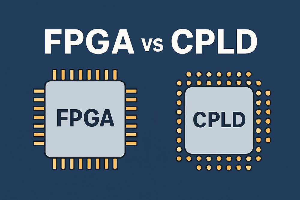
CPLD vs FPGA: Which Programmable Logic Device Fits Your Design?

Short answer: Choose a CPLD-class device when the design demands instant-on, deterministic, low-complexity supervisory or glue logic. Choose an FPGA when the design demands high-density parallel compute, embedded DSP/MAC throughput, rich memory buffering, and high-speed serial connectivity. The decision hinges less on raw speed and more on configuration volatility, timing determinism, power architecture, board-level BOM overhead, and modern lifecycle reality.Executive Summary & Quick Engineering Decision FrameworkHardware designers comparing CPLDs and FPGAs have traditionally encountered a simple density-versus-determinism trade-off. A Complex Programmable Logic Device historically implemented modest logic functions through coarse-grained macrocells with deterministic timing and single-supply board requirements. A Field-Programmable Gate Array provided far greater logic capacity and dedicated arithmetic blocks at the cost of volatile configuration, multi-rail power sequencing, and place-and-route timing complexity.That architectural distinction remains useful, but it is no longer sufficient. Many classic pure macrocell CPLDs are end-of-life or not recommended for new designs, while modern single-chip Flash-based micro-FPGAs now fill the instant-on supervisory role. The selection question has therefore shifted: which programmable-logic architecture minimizes system-level risk while satisfying capacity, timing, and power constraints?Architectural Comparison MatrixComparison ParameterClassic CPLD / Flash-PLD ClassFull-Featured SRAM FPGAModern Single-Chip Flash FPGALogic fabricMacrocell / AND-OR product-term arraysConfigurable Logic Blocks (CLBs) with distributed LUTsLUT-based fabric with on-chip non-volatile configuration memoryConfiguration volatilityNon-volatile internal Flash/EEPROMVolatile SRAM; requires external boot FlashNon-volatile on-chip FlashPower-on latencyInstant-on (microsecond regime)Bitstream boot transfer (milliseconds to seconds)Sub-millisecond to near-instant-onTiming behaviorDeterministic, uniform pin-to-pin propagation delayPlace-and-route dependent; requires iterative timing closurePredictable, though routing-dependent within a single chipDedicated hard IPMinimal or noneDSP slices, Block RAM, PLLs, high-speed SerDesVaries by family; some include PLLs, ADC, and embedded Flash memoryPower architectureSingle-supply or simple dual-rail, low quiescentMulti-rail core/aux/IO PMIC sequencing, higher static leakageSingle-supply or simplified multi-railTypical logic capacityTens to hundreds of macrocellsThousands to millions of LUTs / Logic ElementsHundreds to tens of thousands of LUTsPrimary application fitPower sequencing, bus bridging, interrupt management, glue logicVideo processing, software-defined radio, networking, AI accelerationBoard management, secure boot, mixed-signal supervisionSilicon Selection Rule of ThumbUse this sequence before committing to any device family:Estimate true logic capacity. If the design needs more than roughly a few thousand flip-flops, a classic macrocell CPLD will likely fail capacity.Identify the cold-boot supervisor requirement. If no configured device can be safely released from reset until power rails are stable, an instant-on programmable-logic device must exist on the board.Inventory specialized hardware needs. Design sections requiring DSP MAC units, large Block RAM, or transceiver channels point directly to an FPGA.Audit the power sequencing architecture. A single-rail system tolerant to slow ramp behavior can accept a simpler device; a multi-rail SoC or high-density FPGA needs sequenced enable control.Check the vendor lifecycle status for every candidate part before schematic freeze. Do not rely on legacy CPLD families still appearing in old application notes or distributor search results.Silicon Fabric Architecture: Coarse Macrocells vs. Fine-Grained Look-Up TablesThe CPLD Logic StructureClassic CPLDs descend directly from programmable array logic and programmable logic arrays tracing back to the PAL/PLA era. The internal fabric is built around wide AND-OR product-term arrays feeding configurable macrocells. Each macrocell typically contains a flip-flop, polarity control, and feedback paths into the centralized interconnect matrix.This architecture is optimized for wide fan-in boolean equations. A 32-input address decode, for example, can be evaluated in a single uniform macrocell cycle without passing through multiple cascaded LUT stages. The wide product-term structure is the reason CPLDs have historically been favored for address decoding, bus arbitration, interrupt merging, and state machines with modest sequential depth[1].The limitation is equally architectural. Product-term resources are coarse and consumed inefficiently by arithmetic-heavy logic such as multipliers, barrel shifters, or wide addition trees. Attempting to build a 32-bit multiply-accumulate path inside a macrocell fabric quickly exhausts available product-term budget and yields poor performance.The FPGA Logic StructureFPGAs use an island-style architecture built around fine-grained Configurable Logic Blocks. Each CLB contains multiple Look-Up Tables, commonly with four or six inputs, paired with dedicated storage elements and local routing multiplexers. The LUT truth-table implementation supports arbitrary combinational logic within the LUT's input width; wider logic is decomposed across multiple cascaded LUTs connected through segmented routing channels.This fine-grained fabric scales far more gracefully for complex sequential state machines, deeply pipelined arithmetic datapaths, and dense parallel processing. The presence of dedicated carry chains, synchronous reset networks, and hierarchical clock distribution enables high-frequency datapath implementations that would be impractical in a coarse macrocell fabric.The trade-off is routing complexity. The segmentation of the FPGA interconnect means intermediate signals travel through programmable switch matrices whose electrical parasitics depend on placement and routing congestion. That reality gives rise to the timing-closure burden discussed in a later section.Architectural Trade-OffArchitectureStrengthsWeaknessesMacrocell product-termWide fan-in decoding, uniform delay, simple timing modelCoarse granularity, poor arithmetic efficiency, limited embedded IPLUT/CLB fabricFine granularity, excellent arithmetic and datapath scaling, integrated DSP/BRAMRouting-dependent delay, timing closure effort, larger fabric overheadComparison of coarse CPLD fabric versus fine-grained FPGA fabricConfiguration Memory, Volatility, and the "First-to-Wake" Power Sequencing ImperativeConfiguration Storage MechanismsThe divergence in configuration memory is one of the most consequential differences between CPLD-class devices and SRAM FPGAs.A classic CPLD stores its logic configuration in internal non-volatile EEPROM or Flash. The device wakes immediately once the supply rail stabilizes. There is no external configuration clock, no bitstream interface, and no boot memory component.A conventional SRAM-based FPGA stores its logic configuration in volatile SRAM latches that lose state at power-down. The configuration bitstream resides in an external SPI NOR Flash or QSPI memory and must be streamed into the FPGA on every power cycle. That process consumes milliseconds to seconds depending on bitstream size and configuration interface speed.The "First-to-Wake" Hardware ImperativeThe engineering consequence is deceptively simple: a volatile FPGA or complex SoC cannot manage its own power-up sequence. Before configuration is loaded, the FPGA's I/O pins are undefined and its internal fabric cannot run the power-rail sequencing state machine needed to safely bring up the board.This is where the CPLD-class device earns its place on the modern PCB. Acting as a board-management controller, an instant-on programmable-logic device can:Assert enable signals to PMIC regulators in the correct orderMonitor power-good flags from each railEnforce monotonic voltage ramp behaviorHold the main processor or FPGA in reset until all supplies are stable and the system clock is validDeassert reset and release the main compute device only after Boot-up requirements are satisfiedETH Zurich research on declarative power sequencing using CPLDs demonstrates this precise application[5]: deterministic state-machine control over power-rail enable and reset scheduling in complex compute platforms.Hardware Security and IP ProtectionConfiguration storage architecture also has direct security implications. An SRAM FPGA's bitstream travels over an exposed board-level SPI or QSPI bus, creating a point where the configuration image can be passively sniffed or actively manipulated. Modern SRAM FPGAs mitigate this through bitstream encryption and authentication keys, but the attack surface remains.A CPLD or Flash-based PLD stores configuration entirely on-chip, with no external boot bitstream to intercept. The non-volatile configuration memory is a security-relevant feature in systems requiring IP protection or resilient boot behavior.Verified Modern Instant-On ExampleThe Lattice MachXO3 family demonstrates the modern Flash-PLD approach: per the Lattice MachXO3 datasheet, sub-1 ms wake-up directly from on-chip non-volatile Flash across densities from 640 to 9,400 LUTs and up to 384 I/O pins. Similarly, per the Intel MAX 10 device overview, Intel MAX 10 single-chip FPGAs integrate on-die Configuration Flash Memory and offer dedicated Instant-On modes requiring supply ramp rates within 3 ms to wake without external boot bitstream latency.These specifications matter because they prove the CPLD-style instant-on role is being fulfilled by modern Flash-based single-chip architectures rather than legacy macrocell parts.Timing Determinism & Routing: Continuous Interconnects vs. Place-and-Route ComplexityCPLD Timing PredictabilityClassic CPLDs use a centralized, continuous routing matrix that connects all macrocell outputs and inputs through fixed-length interconnect paths. This topology produces a uniform pin-to-pin propagation delay that is largely independent of where a particular logic function is physically placed within the device.The engineering benefit is timing predictability. An asynchronous address decoder, a reset-merge circuit, or a bus bridge built in a CPLD exhibits consistent delay characteristics across the full operating temperature and voltage range. There are no routing congestion surprises because the routing matrix is not segmented.FPGA Routing RealitiesFPGAs replace the continuous interconnect with segmented routing channels and programmable switch matrices. Signals travel across variable lengths of metal interconnect, pass through multiple switch boxes, and suffer RC delay contributions that depend on physical placement and the degree of routing congestion in the critical path.Consequently, FPGA timing cannot be accurately predicted during schematic design. Engineers must run iterative Static Timing Analysis, apply physical synthesis constraints, and repeatedly place-and-route the design to close timing. A critical path that meets timing at 90% utilization may fail at 95% utilization when routing resources become scarce.Engineering ImpactThe timing-determinism difference has direct consequences for design verification. A hard real-time bus bridge in a CPLD requires fewer simulation cycles and fewer board-level re-spins because the timing model is fixed by architecture. The same function implemented in an FPGA demands careful constraint definition, timing-closure iterations, and re-verification after every logic change.Timing AttributeCPLD-Class DeviceSRAM FPGADelay modelDeterministic, uniformRouting-dependent, variableTiming predictionAvailable at schematic stageRequires post-PnR analysisRace condition risk in async logicLowElevated without careful constraintVerification burdenLowSignificant iterative STAPower Dissipation Dynamics: Quiescent Leakage vs. High-Speed Dynamic SwitchingMathematical Power ModelTotal power consumption in CMOS programmable logic follows the standard formulation:Ptotal=Pstatic+PdynamicPdynamic=CPD·VCC2·f·NSWwhere CPD is power dissipation capacitance, VCC is the core supply voltage, f is the switching frequency, and NSW is the number of switching nodes.Static Power and Quiescent OverheadThe static component is where SRAM FPGAs and CPLD-class devices diverge sharply. An SRAM FPGA must maintain configuration state in thousands or millions of SRAM cells even when no useful logic is switching. High-speed transceiver bias circuits, PLL analog blocks, and configuration control logic all draw quiescent current. This baseline static leakage exists independent of user design activity.Low-density CPLDs and Flash-PLDs, by contrast, can enter extremely low quiescent states because their non-volatile configuration memory does not require continuous latch power to retain state. When the design demands a wake-up supervisor that stays powered during system sleep, this low-standby characteristic is directly relevant.Dynamic Power Scaling Under Clock LoadDynamic power is where simplistic comparisons between CPLDs and FPGAs break down. A CPLD toggling wide product-term arrays at high frequency draws substantial dynamic current because wide internal nodes swing simultaneously across the routing matrix. A large SRAM FPGA toggling only a small portion of its fabric may dissipate less dynamic power than expected, but its static leakage remains present regardless of utilization.The practical implication: architectural power claims are meaningless without specifying clock frequency, toggle rate, logic utilization, and supply voltage. Use vendor power estimation tools and application notes to calculate device-specific thermal budgets before making a selection decision.Power scaling: CPLD static leakage versus FPGA dynamic switchingTotal Cost of Ownership & PCB Complexity: The Hidden BOM Overhead of FPGAsBeyond Silicon CostComparing bare silicon prices between a CPLD and an entry-level FPGA is misleading because the supporting component bill-of-materials differs dramatically.BOM FactorCPLD-Class DeviceSRAM FPGAConfiguration memoryNone requiredExternal SPI/QSPI NOR FlashPower suppliesSingle-rail or simple dual-railMulti-rail: core, I/O, aux, possibly transceiver railPower management ICDiscrete LDO or simple regulatorMulti-output PMIC with sequencingClockingSimple crystal or RC oscillatorLow-jitter differential oscillator often required for transceiversDecouplingBasic decoupling per I/O bankHigh-frequency capacitor arrays across multiple railsPCB layer count2–4 layers feasible6–12+ layers common for BGA fanoutPackage mountingHand-solderable QFP/QFN/TSSOPFine-pitch BGA requiring reflow and possible HDIPCB Fabrication and Layout ConstraintsClassic CPLDs and small Flash-PLDs are frequently available in low-pin-count, hand-solderable packages well suited to 2- to 4-layer PCBs. This simplifies prototyping and low-volume production.SRAM FPGAs, especially mid-range and high-density families, are packaged in fine-pitch BGAs that require high-layer-count stackups, controlled-impedance routing, and sometimes blind/buried microvias for breakout. The result is higher fabrication cost, longer layout cycles, and more complex design reviews.Package TypeTypical Pin CountPCB ImplicationsCPLD QFP/QFN44–144 pins2–4 layer PCB feasible, manual rework possibleFPGA Fine-Pitch BGA256–1,760+ balls6–12+ layer PCB, HDI routing, reflow-only assemblyThe Modern Supply Chain Reality: CPLD Obsolescence vs. Single-Chip Flash FPGAsWhy Legacy Guides and Current Answers DisagreeEngineers researching CPLD vs FPGA today encounter conflicting information. Some older application notes and tutorials still recommend classic 5V or 3.3V macrocell CPLD families that are no longer viable for new designs. Meanwhile, procurement catalogs increasingly use the term "CPLD" to refer to single-chip Flash-based micro-FPGAs with LUT fabrics.This lifecycle gap is not merely academic. Designing a legacy macrocell CPLD into a long-lifecycle industrial, defense, or medical product carries direct supply-chain risk.The Verified Lifecycle RealityAMD issued Product Discontinuation Notice XCN23009, dated January 1, 2024, with a final Last Time Buy on June 29, 2024. That notice officially terminates pure macrocell CPLD families including the XC9500XL, CoolRunner XPLA 3, and CoolRunner II lines, as well as legacy Spartan-II and Spartan-3 FPGAs, with no direct drop-in replacements.This notice provides concrete evidence for a broader industry pattern: the pure AND-OR macrocell CPLD architecture has largely exited mainstream production. Engineers evaluating "CPLD vs FPGA" must therefore distinguish between historical macrocell parts and modern single-chip Flash programmable devices marketed under similar names.The Rise of Modern Single-Chip Flash-Based Micro-FPGAsThe practical replacement for legacy macrocell CPLDs is the modern single-chip Flash micro-FPGA. Families such as Intel MAX 10, Lattice MachXO2/MachXO3/MachXO5, and Microchip IGLOO2 combine non-volatile on-chip configuration memory with instant-on microsecond boot, single-supply operation, and flexible LUT-based logic fabrics.These devices are not merely shrunk FPGAs. Per the Intel MAX 10 device overview, the MAX 10 family specifically integrates on-die Configuration Flash Memory and 12-bit 1 MSPS SAR ADCs, allowing a single chip to wake immediately, supervise power rails, and monitor analog telemetry without an external boot PROM. The MachXO3 family, as noted earlier, achieves sub-1 ms instant-on across up to 9,400 LUTs per the Lattice MachXO3 datasheet.Practical Migration GuidanceWhen updating a legacy design or starting a new hardware revision:Search for lifecycle status by exact part number, not by architecture family name.Treat every legacy CPLD appearing in an old schematic as a redesign candidate.Evaluate Flash micro-FPGA families for both capacity and instant-on suitability.Do not assume a "CPLD" search result is an active macrocell product. Verify against the manufacturer's current product catalog and PCN history.Engineering Selection Framework: When to Choose Which ArchitectureOption A: CPLD-Class Device or Single-Chip Flash-PLDBest for: Board supervisory logic, multi-rail power sequencing, interface level-shifting, wide address decoding, bus arbitration, and hardware-enforced fail-safe functions.Key strengths:Microsecond cold-boot latency when system power stabilizesDeterministic pin-to-pin propagation delay for asynchronous control pathsMinimal BOM overhead: no external configuration memory requiredSimple 2–4 layer PCB layout with hand-solderable packagesNon-volatile on-chip configuration protects IP and prevents bitstream interceptionKey drawbacks:Limited logic density relative to FPGAs; macrocell fabrics in particular cannot scaleMinimal or no dedicated DSP blocks, Block RAM, or high-speed transceiversPoor efficiency for wide arithmetic, multipliers, or deeply pipelined datapathsWho should NOT choose this option: Designs requiring audio/video processing, large packet buffering, multi-gigabit SerDes, complex math acceleration, or dense parallel compute.Option B: Full-Featured SRAM FPGABest for: Digital Signal Processing, multi-gigabit networking, computer vision, software-defined radio, AI inference at the edge, and embedded soft-core or hard-core processor SoCs.Key strengths:Massive parallel compute capability and reconfigurable datapath pipeliningRich dedicated hard IP: DSP slices, Block RAM, PLLs/MMCMs, PCIe/Ethernet transceiversScalable logic capacity across multiple density tiersWide ecosystem of vendor synthesis and verification toolsKey drawbacks:Higher static leakage current due to large configuration latch arraysMillisecond-level boot latency requiring external SPI flashComplex multi-rail PMIC requirements with controlled sequencingLengthy timing closure cycles requiring iterative STAFine-pitch BGA packages driving high-layer-count PCB designsWho should NOT choose this option: Designs needing simple reset sequencing, discrete GPIO expansion, low-cost single-rail battery operation, or minimal board complexity.Alternative Silicon Boundary AnalysisProgrammable logic is not always the right answer. Two adjacent technologies deserve explicit consideration.Ultra-low-power MCU. When the control path is inherently sequential and execution latencies in the microsecond range are acceptable, a small MCU may provide equivalent system supervision at lower cost and lower active power. The MCU's interrupt latency and software boot time must be carefully verified against the system's power-sequencing requirements.Configurable mixed-signal ICs. For very simple glue logic, analog comparator monitoring, and basic power-sequencing tasks, devices such as the Renesas GreenPAK SLG46826 offer an alternative. Per the Renesas SLG46826 datasheet, the SLG46826 provides dual-rail voltage translation supporting VDD from 2.3 V to 5.5 V and VDD2 from 1.71 V to 5.5 V, four rail-to-rail analog comparators, and programmable delay macrocells in a 2.0 mm × 2.2 mm 14-pin STQFN package. When the logic requirement fits within this class of device, the BOM overhead and board space can be substantially lower than even a small CPLD.Common Hardware Selection MistakesOver-specifying an FPGA for simple GPIO expansion — The result is unnecessary layout complexity, multi-rail power sequencing burden, and a larger PCB stackup.Under-specifying a CPLD for math-heavy state machines — Wide arithmetic and multiplier functions exhaust macrocell product-term resources rapidly.Ignoring cold-boot timing gaps — A design that releases the main processor from reset before power-good confirmation can exhibit destructive latch-up or intermittent boot failures.Assuming legacy CPLD availability — Failure to verify lifecycle status results in parts that become unobtainium mid-design.Treating bare silicon cost as total cost — A low-cost FPGA that requires a $6 PMIC, external flash, and a 10-layer PCB may cost more at the board level than a single-supply CPLD.Frequently Asked QuestionsAre pure macrocell CPLDs still being manufactured for new designs?Most pure AND-OR macrocell lines are legacy, NRND, or EOL. AMD's Product Discontinuation Notice XCN23009 (2024) officially terminated the XC9500XL, CoolRunner XPLA 3, and CoolRunner II families with a final Last Time Buy of June 29, 2024. New commercial designs primarily use Flash-based single-chip micro-FPGAs that provide instant-on, single-chip operation using modern LUT fabrics. Always verify lifecycle status against the manufacturer's current product catalog.Can an FPGA directly replace a CPLD on an existing PCB?Rarely as a drop-in replacement. SRAM FPGAs generally require different package pinouts, additional core voltage rails, and external configuration memory. A Flash-based micro-FPGA may come closer functionally, but package and electrical incompatibilities typically require a board revision. Any replacement candidate must be validated against the original schematic's voltage domains, pin mapping, and timing constraints.What are the primary technical disadvantages of pure CPLDs?The coarse macrocell granularity makes them inefficient for wide arithmetic and complex datapath processing. They also lack integrated Block RAM and DSP slices, which prevents execution of complex data processing pipelines. In addition, many classic macrocell families are no longer available for new designs.How does a CPLD differ from a fast microcontroller in control paths?CPLDs provide true hardware-level concurrency with nanosecond-scale deterministic propagation delays. MCUs execute sequential software instructions with interrupt latencies in the microsecond range. A CPLD's parallel hardware responds to input changes without software overhead, making it suitable for combinatorial decode, asynchronous bus arbitration, and hardware-enforced fail-safe logic that cannot tolerate software boot time.Difference Between CPLD and FPGA | Programmable Logic Devices | Digital Electronics in EXTCHardware Engineering Verification Checklist Before Silicon ProcurementUse this checklist before freezing the schematic or signing the BOM.[ ] Power supply count and sequencing — Verify whether the device requires single-rail operation or multi-rail PMIC sequencing. Identify every enable, soft-start, and power-good input.[ ] Cold-boot startup latency — Confirm the exact time-to-active from voltage threshold to operational state. For Flash micro-FPGAs, verify the instant-on spec against the system's power-sequencing target.[ ] Propagation delay constraints — Confirm worst-case pin-to-pin delay across operating temperature and speed grades for asynchronous decode paths.[ ] I/O bank compatibility and hot-socketing — Verify voltage tolerance (1.2 V, 1.8 V, 2.5 V, 3.3 V), fail-safe clamps, and floating-pin behavior during power ramping.[ ] Vendor lifecycle status and PCN history — Verify active production status and review recent Product Change Notifications. For any legacy part, check for discontinuation notices before committing the design.[ ] Package fanout and PCB layer feasibility — Check package pitch (e.g., 0.5 mm BGA vs. 0.8 mm QFP) to confirm stackup layer count, via technology, and fabrication cost.[ ] Thermal envelope and static leakage — Calculate worst-case junction temperature based on maximum quiescent leakage and switching frequency. Use the vendor's power estimator if available.[Sources and references used for this guideCPLD - What is the difference between CPLDs and FPGAs?Source type: official company documentationUsed for: Canonical definitions of macrocell product-term architectures versus Look-Up Table (LUT) FPGA fabrics, non-volatile internal routing, and configuration memory distinctions.Caution: Vendor support documentation representing AMD/Xilinx architectural classifications; focus on structural silicon mechanisms rather than specific legacy part recommendations.Hot-Socketing & Power-Sequencing Feature & Testing for Altera DevicesSource type: official company documentationUsed for: Technical analysis of PLD power-up sequencing, hot-socketing capabilities, I/O pin behaviors during supply ramping, and hardware supervisory roles.Caution: Official Altera/Intel technical collateral; focuses on device reliability and power behavior rather than third-party competitive comparisons.Power-Aware FPGA DesignSource type: official company documentationUsed for: Modeling static leakage current, dynamic switching dissipation, clock gating, and power optimization strategies across programmable logic fabrics.Caution: Vendor whitepaper emphasizing Microchip's Flash-based FPGA efficiency; calculations apply broadly to CMOS logic but narrative highlights proprietary low-power advantages.CMOS Power Consumption and CPD CalculationSource type: official company documentationUsed for: Mathematical modeling of CMOS dynamic power consumption, internal capacitance calculation, and frequency-dependent power scaling.Caution: Foundational semiconductor physics application note; establishes universal formulas (CV2f) rather than programmable device selection heuristics.Declarative Power Sequencing using a CPLDSource type: research sourceUsed for: Academic and experimental validation of CPLD deterministic timing in real-time power supply rail sequencing and fault management in complex compute platforms.Caution: Academic research paper focused on specific power management implementations; demonstrates determinism advantages but does not cover general-purpose FPGA compute workloads.Models for reducing power consumption in CPLD and FPGA devicesSource type: research sourceUsed for: Comparative academic study on static leakage versus dynamic power dissipation under varying clock frequencies in programmable logic.Caution: Conference paper; provides comparative modeling data but utilizes specific older generation test benches.CPLD vs FPGA: Key Differences and How to ChooseSource type: reputable professional sourceUsed for: Engineering overview of macrocell vs LUT density, pin-to-pin propagation delay differences, and high-level selection criteria.Caution: Tertiary engineering publication; serves as a structuring reference for design trade-offs, but specific numerical figures must be cross-checked against component datasheets.GreenPAK vs FPGA vs CPLD: Which Is Right for Your Design?Source type: vendor articleUsed for: Board-level PCB design trade-offs, package footprints, and boundary comparisons between programmable logic, microcontrollers, and mixed-signal arrays.Caution: EDA vendor blog; useful for PCB layout and routing perspective, but contains commercial product references.
Kynix On 2026-08-25   38
Sensor

Gas Sensors for IoT: Types, Key Specs, and Selection Guide

The short answer: there is no universal gas sensor for IoT. Gas sensor selection is a coupled engineering trade-off between sensing physics, power budget, temperature/humidity stability, response time, measurement selectivity, and field replacement cost.As a practical starting point for gas sensor IoT selection:Battery-powered toxic gas detection for CO, H₂S, NO₂, or O₂ usually points to electrochemical sensors operating at microampere-level signals.Long-life CO₂ or methane measurement with stable baselines usually points to non-dispersive infrared (NDIR) sensors.Broad indoor air quality, total VOC trend, or smoke screening usually points to metal-oxide semiconductor (MOS/MOX) sensors with duty-cycled micro-hotplates.Flammable gas detection across 0–100% LEL usually points to catalytic bead pellistors or infrared sensors on mains/industrial power rails.The rest of this guide breaks down why those choices hold, where they fail, and what to verify before finalizing a design.1. The 5-vector IoT gas sensing decision frameworkBefore selecting a part number, predefine five system vectors. Most failed gas-sensor designs come from fixing one vector and ignoring the others.Decision vectorWhat to freeze earlyWhy it changes the architectureTarget gas and measurement envelopeSpecific gas, concentration range, resolution, detection limitDetermines whether redox, infrared absorption, or chemiresistive physics is appropriatePower and energy sourceMains, LiSOCl₂, Li-ion, energy harvesting, peak-pulse capabilityRules out continuous heater devices or requires aggressive duty cyclingEnvironmental profileTemperature, humidity, dust, water spray, interfering gasesDrives enclosure design, filters, compensation, and sensor lifetimeDynamic performance and lifespanRequired T90, warm-up time, acceptable drift, service intervalSeparates consumable electrochemical cells from long-life optical or solid-state optionsInterface and total cost of ownershipRaw analog vs. digital module, field replacement strategy, calibration accessChanges analog front-end, firmware, PCB layout, and service architectureA useful decision order for embedded teams:Identify the gas. Is it toxic, flammable, infrared-active, or broad VOC?Define the power envelope. Can the node deliver hundreds of milliwatts, or only microamps?Decide whether the output must be absolute concentration. For safety compliance or ppm-level controls, avoid broad MOS as the sole signal.Assess environment extremes. High humidity, condensing atmospheres, and low oxygen environments directly remove some technologies.Model total service cost. A sensor that must be replaced every two years should be field-swappable.2. Sensor Topologies Compared: Physics, Performance Matrices, and Application BoundariesThe main IoT-relevant sensor classes are electrochemical, NDIR, MOS/MOX, and catalytic bead pellistors. They do not compete directly; each occupies a different physical and application boundary.Sensing technologyPrimary physical principleTypical target gasesPower consumptionResponse timeSelectivity and cross-sensitivitiesOperating lifespanRelative BOM cost tierElectrochemical (EC)Redox reaction at electrodes produces proportional currentCO, H₂S, NO₂, O₂, SO₂Sub-mW continuous; nanoampere-to-microampere signal outputSeconds to minutes, depending on filter, electrolyte, and temperatureHigh for target gas; cross-sensitivity to hydrogen, some VOCs1–3 years typical; 12–18 months for reactive acid gasesMediumNDIRGas absorbs infrared light at specific wavelengths; concentration derived from Beer-Lambert lawCO₂, CH₄, infrared-active hydrocarbonsLow average power via pulsed IR source; high peak supply currentTens of seconds to minutes depending on chamber volumeHigh for infrared-active gas; immune to catalytic poisoning5–10+ years typicalHighMOS/MOXHeated metal-oxide film changes resistance during gas adsorptionBroad VOCs, smoke, combustible gas indicationHigh continuous heater power; low average power with MEMS duty cyclingFast with MEMS micro-hotplates; slower with ceramic heatersLow; responds broadly to VOCs, humidity, and temperatureModerate; can be poisoned by silicones and heavy solventsLow to mediumCatalytic bead / pellistorCatalytic oxidation on heated bead changes bridge resistanceFlammable gases, 0–100% LEL140 mW to 190+ mW per bead pair continuousFast, typically secondsBroad combustible response; requires oxygen2–3 years typicalLow to mediumGas Sensor Technology Comparison: Physics and PowerElectrochemical sensors: microampere toxic gas detectionElectrochemical gas sensors are the closest fit for battery-operated single-gas toxic monitoring. The target gas diffuses through a barrier into a liquid or gel electrolyte and reacts at the working electrode. The resulting redox current is proportional to gas concentration.For industrial toxic cells, output signals are typically in the nanoampere-to-microampere range. For example, Alphasense CO, H₂S, and O₂ amperometric cells generate linear current outputs, with oxygen cells often producing roughly 80–120 μA in air and zero-baseline currents below 2.5 μA at 20°C. That current must be conditioned by a high-impedance transimpedance amplifier before the MCU ADC.Best for: battery-powered CO, H₂S, NO₂, and O₂ monitoring.Main weaknesses: limited consumable lifespan, sensitivity to extreme humidity, temperature-dependent output, and the need for periodic recalibration.Do not choose EC when: the deployment is a permanently sealed, zero-maintenance outdoor device; when the gas is primarily a broad VOC mixture; or when the environment exceeds the cell's rated humidity or temperature envelope.NDIR sensors: drift-resistant optical measurementNDIR sensors operate by pulsing an infrared source through an optical chamber and filtering for a narrow absorption wavelength. CO₂ absorbs near 4.26 μm, while methane and many hydrocarbons absorb in the 3.3–3.4 μm region. The gas reduces detected optical intensity; concentration is calculated from that attenuation.NDIR is highly selective for infrared-active gases and is not subject to the same chemical poisoning mechanisms as pellistors or MOS sensors. However, homonuclear diatomic molecules such as O₂, N₂, and H₂ do not absorb infrared light in the same useful way and cannot be measured with standard NDIR. These fundamental optical principles are well documented in technical comparisons of NDIR vs electrochemical gas sensors[8].Best for: indoor CO₂ monitoring, greenhouse CH₄ measurement, ventilation control, and long-life environmental nodes.Main weaknesses: higher device cost, larger optical path, peak-current demand during emitter pulses, and condensation risk in humid chambers.Do not choose NDIR when: measuring oxygen depletion, hydrogen leaks, or non-infrared-active gases, or when the BOM cannot support an optical cell.MOS/MOX sensors: high-sensitivity chemiresistorsMOS sensors rely on a heated polycrystalline metal-oxide layer, often tin oxide or tungsten oxide. Gas adsorption changes the grain-boundary resistance. The device is typically heated to 200°C–400°C.MOS is attractive because it is small, low cost, and extremely sensitive to many VOCs. But it is not a precise single-gas analyzer. Humidity changes, temperature swings, and common household VOCs can produce large baseline changes.A useful example is the Bosch BME688 MEMS gas sensor. In its standard gas-scan mode, it draws about 3.9 mA, drops to 0.9 mA in low-power mode, and falls to roughly 90 μA in ultra-low-power mode. Its fast thermal response can reach T33–63% in under one second, making it suitable for short duty-cycled measurements—but that speed depends on the device being allowed to reach thermal and surface equilibrium before sampling.Best for: qualitative IAQ indices, broad VOC trend monitoring, odor detection, and early smoke/combustion screening.Main weaknesses: poor selectivity, humidity drift, non-linear response, and baseline aging.Do not choose MOS when: regulatory-grade ppm accuracy is required for a single toxic gas, or when the device must run continuously on a small coin cell without duty cycling.Catalytic bead pellistors: flammable gas LEL monitoringPellistor sensors are thermal catalytic devices. A matched pair of heated beads sits in a Wheatstone bridge. Combustible gas oxidizes on the active catalytic bead, raising its temperature and changing its resistance. The output is proportional to the flammable gas concentration across the 0–100% lower explosive limit range.Pellistor operation requires constant bead heating to approximately 450°C–500°C, leading to continuous power draw from about 140 mW to more than 190 mW per bead pair. The catalytic reaction also depends on adequate oxygen, typically at least 15%–21% ambient O₂. Typical pellistor service life is around 2–3 years.Best for: mains-powered or industrial combustible gas detection, fixed safety nodes, and 4–20 mA loop systems.Main weaknesses: high continuous power, oxygen dependency, and vulnerability to permanent poisoning by airborne silicones, sulfur compounds, or lead.Do not choose pellistors when: the node is battery-powered, deployed in oxygen-depleted or inert atmospheres, or expected to operate without field service for many years.3. Power Architecture and Edge Battery OptimizationPower architecture often decides the sensor class before accuracy does.Electrochemical cells are the least demanding in continuous current. They operate in the nanoampere-to-microampere signal range and require only low-power analog conditioning. The power budget is dominated by the TIA, ADC, MCU, and communication radio rather than the sensor itself.NDIR sensors look low-power on average but can demand significant peak current. The Sensirion SCD40/SCD41 photoacoustic NDIR CO₂ family, for example, operates from 2.4 V to 5.5 V and draws an average of about 15–18 mA in periodic 5-second mode, falling to roughly 3.2–3.5 mA in 30-second low-power mode. However, peak supply current can reach 175–205 mA at 3.3 V, or 115–137 mA at 5 V. Supply ripple must remain below about 30 mV peak-to-peak. This is why NDIR designs often need a low-ESR capacitor, a dedicated LDO, or a hybrid layer capacitor across the battery rail.MOS and pellistor devices are the hardest to run on batteries. A traditional ceramic MOS heater can draw hundreds of milliwatts continuously. MEMS micro-hotplate devices such as the BME688 reduce that substantially by lowering the thermal mass and allowing fast warm-up. Empirical studies of low-power IoT electronic nose nodes confirm that careful power consumption modeling and duty cycling[2] are essential to achieve multi-year battery life with such sensors. A practical duty cycle may look like:Deep sleep: MCU and sensor in lowest quiescent state.Power rail enable: bring up the sensor supply and communication bus.Pre-heat stabilization delay: wait for the hotplate to stabilize before reading.ADC sampling and averaging: take multiple samples with a settled surface.Bus transmission: send the processed reading to the host or radio.Power down: remove sensor power or enter low-power mode.Reading a MOS sensor before thermal equilibrium produces misleading baseline jumps. The pre-heat stabilization time must be included in active-energy calculations; quoting only sleep current is not enough.Duty-Cycled Gas Sensor Power Profile4. Environmental Cross-Sensitivity, Drift, and Signal ConditioningGas sensors are exposed to the same atmosphere as the environment they measure. Moisture, temperature, dust, and interfering gases can corrupt the raw signal.For electrochemical cells, the operational boundary is often around −30°C to +55°C and 5% to 95% RH non-condensing. Below 15% RH, electrolyte desiccation can occur. Above 90% RH, prolonged condensing conditions can flood the cell, absorb water, and damage the internal chemistry. Once the electrolyte is depleted or flooded, no firmware compensation curve can recover the sensor.MOS sensors are especially sensitive to rapid humidity steps. Water vapor competes with target gases for surface sites on the metal-oxide grain boundaries, changing baseline resistance independent of VOC concentration. This is why a sudden bathroom humidity spike or weather front can appear as an indoor air quality event. Research on electrochemical and metal oxide sensors for fire gas detection also highlights these cross-sensitivity and humidity drift[5] effects.Common mitigation techniques include:Hydrophobic ePTFE membranes to block liquid water and dust.Sintered flame arrestors for flammable gas sensors.Co-located temperature and humidity sensors for firmware compensation.Two-dimensional polynomial compensation of raw output against temperature and humidity.Dual-wavelength NDIR optical references to reject source aging and dust buildup.Temperature also changes electrochemical response speed. Lower temperatures tend to slow gas diffusion and electrolyte kinetics, while elevated temperatures can accelerate response and recovery—but may also shorten cell life or shift the baseline.The peer-reviewed gas sensor literature supports these limitations. MOS semiconductor sensors show broad sensitivity but also clear temperature and humidity drift, while electrochemical sensors need stable thermal and humidity boundaries to maintain output linearity.5. Hardware Interface Selection and Edge Firmware IntegrationGas sensors usually reach the MCU through raw analog output, I2C, UART, SPI, or an industrial current loop.InterfaceBest usePractical boundaryKey cautionRaw analogEC cells, many MOS and pellistor outputsShort PCB traces, guarded high-impedance inputsRequires TIA or amplifier, ADC matching, and noise controlI2CFactory-calibrated digital modules, multiple sensors on one busShort runs, typically under 30 cm with 400 pF bus capacitancePull-up sizing depends on bus speed and line capacitanceUARTPoint-to-point remote probe or moduleShielded cable runs of a few metersSimple, but needs level shifting and noise filteringSPIHigh-speed local sensor dataVery short PCB tracesExtra pins and limited slave count4–20 mAIndustrial gas detectors, long field runsLong cable distances in noisy plantsHigher loop power and industrial gateway hardwareDigital gas modules offload much of the analog design. They may include an internal ADC, factory calibration coefficients, and a simple host protocol. But they do not remove firmware responsibilities. The host still needs timeout recovery, bus reset routines, baseline tracking, and startup suppression logic.In firmware, use non-blocking polling instead of blocking delays in the main loop. During power-on, lock out alarm thresholds until the sensor has completed its warm-up sequence; otherwise, the node may emit a false gas alarm before the signal has stabilized. On the cloud side, rate-limit alert events so a sustained high-gas event does not flood the message broker or trigger platform throttling.6. Operational Lifespan, Recalibration Realities, and Critical PitfallsSeveral common claims about IoT gas sensors do not hold up in the field.Misconception: “Electrochemical sensors last 5–10 years maintenance-free.”Most electrochemical cells are consumables. CO or H₂S cells often last around 2–3 years, while reactive acid-gas cells for HF, Cl₂, or SO₂ may last only 12–18 months. The electrolyte depletes or degrades even without target gas exposure. The electrochemical sensing literature confirms these lifespan and degradation[1] characteristics.Misconception: “Automatic Baseline Calibration solves all NDIR drift.”Automatic Baseline Calibration assumes the sensor sees near-background air at some point. In continuously occupied spaces, greenhouses, intensive livestock barns, or 24/7 manufacturing facilities, ABC may treat an elevated CO₂ level as the new baseline and underreport true concentration. In those applications, ABC should often be disabled in firmware and replaced with manual zero/span calibration or a known reference cycle.Misconception: “MOS sensors run easily on coin cells out of the box.”Traditional heated MOS sensors can drain a CR2032 in hours if continuously powered. Only a MEMS hotplate with aggressive duty cycling, or a different battery chemistry with low internal impedance, makes multi-year operation feasible.Misconception: “Multi-gas MOS sensors can report absolute toxic ppm values.”MOS sensors are best treated as qualitative or semi-quantitative. They can support a VOC index or trend output, but they do not provide the single-gas selectivity needed for regulated personal safety monitoring.Pellistor and MOS surfaces are vulnerable to irreversible poisoning. Volatile methylsiloxanes from silicone sealants, adhesives, and lubricants can decompose on the heated sensor surface and deposit solid silica, permanently covering catalytic or sensing sites. That failure mode often appears as an unexplained loss of sensitivity and cannot be fixed by recalibration.A practical field-service architecture uses modular, pre-calibrated, field-swappable sensor cartridges. The cartridge carries the gas-specific cell, calibration data, and interface connector. The node remains reusable, while the consumable element is replaceable.7. Pre-Tapeout Engineering and Sourcing Verification ChecklistUse this before PCB freeze and production sourcing.Hardware and electrical verification[ ] Power rail can deliver NDIR emitter or MOS heater peak current without brownout.[ ] Bypass and bulk capacitance meet the sensor's ripple and transient requirements.[ ] ADC input range matches the analog signal swing; voltage dividers are impedance-checked.[ ] I2C pull-up resistors are sized for bus capacitance and clock speed.[ ] High-impedance analog traces are kept away from switching regulators, RF lines, and high-current paths.[ ] Transimpedance amplifier selected for electrochemical current range and low input bias current.Mechanical and enclosure design[ ] Gas diffusion port is protected from water droplets and dust.[ ] Internal dead volume is small enough to avoid excessive response-time degradation.[ ] Hot components are thermally separated from gas-sensing elements.[ ] Hydrophobic membrane or sintered flame arrestor is present for the intended environment.Firmware and correction logic[ ] Warm-up lockout timer prevents false alarms before sensor stabilization.[ ] Temperature and humidity compensation tables are stored in non-volatile memory.[ ] Communication timeouts, I2C bus resets, and sensor re-initialization routines are implemented.[ ] Cloud alert events are rate-limited.[ ] NDIR ABC logic is evaluated for the deployment background gas profile.Supply chain and lifecycle[ ] Sensor lifetime matches the product warranty and field-replacement plan.[ ] Required safety certifications are verified against the actual sensor module and end product classification.[ ] Alternate pin-compatible sensors are evaluated.[ ] Calibration fixtures and cartridges are defined before volume deployment.8. Frequently Asked Questions (IoT Gas Sensor Selection)Why do MOS gas sensors report false air pollution spikes during sudden humidity changes?Because water vapor adsorbs on the metal-oxide surface and changes the same grain-boundary resistance that target gases change. A rapid humidity step can appear as a VOC spike even when no pollutant concentration changed. Firmware compensation helps, but cannot fully replace proper environmental characterization.Can NDIR sensors detect oxygen depletion or flammable hydrogen leaks?No. NDIR depends on molecular infrared absorption. Homonuclear diatomic molecules such as O₂, H₂, and N₂ lack the required dipole behavior for useful NDIR detection. Oxygen depletion typically requires an electrochemical oxygen cell, while hydrogen leaks may require a suitable electrochemical, MOS, or thermal-conductivity sensor.How does ambient temperature affect electrochemical sensor response time?Temperature changes gas diffusion speed and electrolyte kinetics. In cold environments, diffusion slows and T90 can increase. At elevated temperatures, response and recovery may become faster, but the cell may age more quickly or exhibit baseline shift. The sensor's stated response time should not be treated as constant across the full operating temperature range.What is the difference between qualitative VOC index monitoring and absolute ppm safety sensing?A VOC index is a relative output generated by an algorithm that tracks changing MOS signal patterns against a baseline. It is useful for ventilation control and air-quality trends. Absolute ppm sensing requires a calibrated, gas-specific transducer such as an electrochemical cell or a properly referenced NDIR sensor, especially when safety limits or regulatory exposure levels are involved.How often do IoT gas sensor nodes require physical recalibration in the field?It depends on the technology and gas. Electrochemical toxic gas cells may need several recalibration or replacement checks per year, depending on exposure and environmental stress. NDIR sensors often require less frequent recalibration, especially with a valid baseline strategy. MOS sensors generally rely on firmware baselining rather than absolute ppm calibration and should not be treated as precision safety instruments.Gas Level Monitoring and Alert Using Blynk IOT and ESP8266 | Blynk IOT ProjectsSources and references used for this guideRecent Advances in Electrochemical Sensors for Detecting Hazardous GasesSource type: research sourceUsed for: Electrochemical redox sensing physics, response time dynamics, and low-power transducer mechanisms.Caution: Academic research paper; focuses on experimental sensing materials alongside standard commercial cells.Low-Power and Low-Cost Environmental IoT Electronic Nose Node Power Consumption StudySource type: research sourceUsed for: Empirical power consumption modeling of gas sensor nodes, battery duty-cycling, and thermal operating states.Caution: Node implementation details reflect specific lab architecture; adapt power models to target MCU and battery chemistry.A Comprehensive Review of Advanced Sensor Technologies for Environmental and Gas MonitoringSource type: research sourceUsed for: Taxonomy of gas sensors in IoT, comparative analysis of EC, NDIR, and MOS topologies.Caution: Review paper aggregating broad industry data; verify specific component part numbers against vendor datasheets.IoT-Enabled Gas Sensors: Technologies, Applications, and OpportunitiesSource type: research sourceUsed for: Multi-gas sensor arrays, semiconductor integration, and wireless network interface trade-offs.Caution: Covers high-level IoT system design; requires supplemental electrical schematics for board layout.Research Progress on Electrochemical and Metal Oxide Gas Sensors for Fire Gas DetectionSource type: research sourceUsed for: MOS broad cross-sensitivity, temperature/humidity drift mechanisms, and response speed comparisons.Caution: Focuses heavily on combustion and fire-gas dynamics; apply principles cautiously to ambient IAQ.Comparison of Gas Sensor Technologies for Rapid Fire and Gas DetectionSource type: research sourceUsed for: T90 response time evaluation, ceiling vs. ambient diffusion dynamics, and sensor kinetics.Caution: Empirical data collected in specific fire-testing geometries; evaluate diffusion rates according to enclosure design.Advancements in Smart Electrochemical Gas Sensors for IoT and Wearable IntegrationSource type: research sourceUsed for: Miniaturization of electrochemical cells, microampere power conditioning, and digital edge interfaces.Caution: Covers emerging nano-material transducers; cross-check availability for high-volume commercial manufacturing.NDIR vs Electrochemical Gas Sensors: Key Differences ExplainedSource type: vendor articleUsed for: Comparative operational analysis between optical infrared absorption and chemical redox cells.Caution: Vendor technical publication; useful for application framing but not independent laboratory proof. {"@context":"https://schema.org","@type":"FAQPage","mainEntity":[{"@type":"Question","name":"Why do MOS gas sensors report false air pollution spikes during sudden humidity changes?","acceptedAnswer":{"@type":"Answer","text":"Because water vapor adsorbs on the metal-oxide surface and changes the same grain-boundary resistance that target gases change. A rapid humidity step can appear as a VOC spike even when no pollutant concentration changed. Firmware compensation helps, but cannot fully replace proper environmental characterization."}},{"@type":"Question","name":"Can NDIR sensors detect oxygen depletion or flammable hydrogen leaks?","acceptedAnswer":{"@type":"Answer","text":"No. NDIR depends on molecular infrared absorption. Homonuclear diatomic molecules such as O₂, H₂, and N₂ lack the required dipole behavior for useful NDIR detection. Oxygen depletion typically requires an electrochemical oxygen cell, while hydrogen leaks may require a suitable electrochemical, MOS, or thermal-conductivity sensor."}},{"@type":"Question","name":"How does ambient temperature affect electrochemical sensor response time?","acceptedAnswer":{"@type":"Answer","text":"Temperature changes gas diffusion speed and electrolyte kinetics. In cold environments, diffusion slows and T90 can increase. At elevated temperatures, response and recovery may become faster, but the cell may age more quickly or exhibit baseline shift. The sensor's stated response time should not be treated as constant across the full operating temperature range."}},{"@type":"Question","name":"What is the difference between qualitative VOC index monitoring and absolute ppm safety sensing?","acceptedAnswer":{"@type":"Answer","text":"A VOC index is a relative output generated by an algorithm that tracks changing MOS signal patterns against a baseline. It is useful for ventilation control and air-quality trends. Absolute ppm sensing requires a calibrated, gas-specific transducer such as an electrochemical cell or a properly referenced NDIR sensor, especially when safety limits or regulatory exposure levels are involved."}},{"@type":"Question","name":"How often do IoT gas sensor nodes require physical recalibration in the field?","acceptedAnswer":{"@type":"Answer","text":"It depends on the technology and gas. Electrochemical toxic gas cells may need several recalibration or replacement checks per year, depending on exposure and environmental stress. NDIR sensors often require less frequent recalibration, especially with a valid baseline strategy. MOS sensors generally rely on firmware baselining rather than absolute ppm calibration and should not be treated as precision safety instruments."}}]}
Victoria On 2026-08-19   46
Sensors

MEMS Sensor Accelerometers, Gyroscopes, and Pressure Sensors: Transduction Physics, Noise Modeling, and System Integration

This guide explains the MEMS sensor accelerometer gyroscope landscape for embedded systems engineers and IoT hardware designers, offering an architectural framework for evaluating, integrating, and optimizing these sensors. By analyzing the physical mechanics of silicon microstructures alongside stochastic noise models, sensor fusion algorithms, low-power firmware patterns, and printed circuit board (PCB) layout constraints, this guide bridges the gap between isolated datasheet specifications and reliable, production-grade tracking systems.10-DoF SENSING ARCHITECTUREMEMS ACCELEROMETERMEMS GYROSCOPEMEMS BAROMETRIC PRESSUREProof-mass / springsDifferential comb-capacitanceGravity vector tiltDynamic linear forceResonant drive mass (10 kHz - 40 kHz)Coriolis sensingDynamic angular rateSusceptible to driftFlexible silicon diaphragmReference vacuum cavityCapacitive vs. piezoresistive bridgeSea-level hypsometric equationSub-2 cm vertical resolutionSENSOR FUSION & FILTERINGHigh-Pass Filter (Gyro rate integration) + Low-Pass Filter (Accel gravity tilt vector)Complementary Filter / Madgwick Quaternion AHRS / Extended Kalman Filter (EKF)Barometric vertical velocity integration (Z-axis altitude state update)LOW-POWER FIRMWARE & SYSTEM INTEGRATIONHardware FIFO watermark interrupts (burst I2C / SPI / I3C) to maximize MCU sleepWake-on-Motion (WoM) threshold triggers (< 15 µA low-power mode)PCB mechanical stress isolation & acoustic resonance keep-out (> 9 kHz - 30 kHz)Micro-Electromechanical Transduction: How Silicon Measures Motion and PressureMicro-electromechanical systems (MEMS) convert mechanical stimuli—such as inertial forces, angular momentum, and fluid pressure—into electrical signals using sub-micron silicon structures fabricated via Deep Reactive-Ion Etching (DRIE) and surface micromachining. Furthermore, this section details the transduction physics of MEMS sensor accelerometer gyroscope and pressure devices.MEMS Accelerometer and Gyroscope Silicon MicrostructuresCapacitive MEMS Accelerometers: Proof-Mass Deflection and Comb-Finger DynamicsA capacitive MEMS accelerometer measures linear acceleration through a mechanical mass-spring-damper system. A micro-machined silicon proof mass (m) is suspended above a substrate by flexible silicon suspension tethers acting as springs with an effective stiffness constant (k) and mechanical damping coefficient (c).When an external acceleration (a) acts on the sensor housing, the housing moves relative to the proof mass, displacing the proof mass by a distance Δx governed by Newton's second law and Hooke's law:Δx = (m · a) / kIn visual stress tests and 3D micro-electromechanical models, this central proof mass is flanked by interdigitated movable capacitive fingers that mesh symmetrically between fixed stator fingers. This geometry forms a differential parallel-plate capacitor pair (C1 and C2). Under zero acceleration, the nominal finger gap on both sides is equal (d), yielding identical capacitance:C0 = (ε · A) / dwhere ε is the permittivity of the medium and A is the overlapping surface area of the comb fingers.When linear acceleration deflects the proof mass by Δx, the gap of one capacitor decreases (d − Δx) while the opposing gap increases (d + Δx). According to Analog Devices MEMS design notes, the resulting differential capacitance is expressed as:ΔC = C1 − C2 = εA [ 1 / (d − Δx) − 1 / (d + Δx) ] = 2εA · Δx / (d2 − Δx2)For small deflections where Δx ≪ d, the relationship linearizes:ΔC ≈ 2εA · Δx / d2This differential capacitance change (ΔC) is routed to an on-chip Application-Specific Integrated Circuit (ASIC), where a switched-capacitor charge amplifier and a sigma-delta (ΣΔ) capacitance-to-digital converter (CDC) convert the picofarad- or femtofarad-level shift into a digital word proportional to acceleration.Capacitive sensing measures both dynamic accelerations (such as mechanical shock and vibrations) and static accelerations (such as Earth's gravitational vector g ≈ 9.81 m/s2), allowing 3-axis accelerometers to serve as tilt and inclination monitors[1].Vibrating Structure MEMS Gyroscopes: Coriolis Acceleration and Mode-MatchingA MEMS gyroscope does not measure absolute orientation angle directly. Instead, it measures angular rate of rotation (Ω, expressed in degrees per second, dps, or radians per second, rad/s) by harnessing the Coriolis effect on a vibrating proof mass.The sensor contains an internal silicon frame driven into continuous primary mechanical resonance oscillation along a drive axis (X) at a velocity v(t) = v0 sin(ωdrive t). Drive-mode resonance frequencies in modern consumer and industrial gyroscopes typically operate between 10 kHz and 40 kHz.When the sensor undergoes angular rotation at rate Ω around an axis perpendicular to the drive oscillation (Z), the moving mass experiences an apparent Coriolis acceleration (ac) directed along the orthogonal sense axis (Y):ac = −2(Ω × v)The corresponding Coriolis force acting on the proof mass (m) is:Fc = −2m(Ω × v)This orthogonal force drives a secondary mechanical sense mode, causing micro-scale displacement of secondary sensing comb fingers. The resulting differential capacitance shift on the sense axis is directly proportional to the applied angular velocity Ω.To achieve high sensitivity, the mechanical quality factor (Q) of the sense structure must be maximized by eliminating viscous air damping. As established in MDPI micromachines research, MEMS gyroscope dice are vacuum-sealed at the wafer level[6] using eutectic or glass-frit bonding to maintain cavity pressures below 10−2 mbar, routinely achieving vacuum quality factors Q > 10,000.MEMS Barometric Pressure Sensors: Piezoresistive Bridges vs. Capacitive DiaphragmsMEMS barometric pressure sensors detect static ambient atmospheric pressure by measuring the mechanical deflection of an etched silicon diaphragm suspended over an engineered reference vacuum chamber.Piezoresistive Sensing DiaphragmCapacitive Sensing DiaphragmMechanism: Atmospheric pressure deforms silicon membrane containing four implanted piezoresistors wired in a Wheatstone bridge circuit (R1 - R4).Response: ΔR / R = πlσl + πtσtMechanism: Atmospheric pressure deflects a flexible conductive silicon diaphragm relative to a fixed rigid metal plate across a sealed vacuum cavity.Response: C = (ε · A) / dTwo transduction architectures dominate modern embedded systems:Piezoresistive Pressure SensorsPiezoresistive sensors use four piezoresistors implanted into the edges of the silicon diaphragm and connected in a balanced Wheatstone bridge circuit. When atmospheric pressure deflects the membrane, localized mechanical stress (σ) alters the electrical resistivity (ρ) of the silicon matrix via the piezoresistive effect:ΔR / R = πlσl + πtσtwhere πl and πt represent the longitudinal and transverse piezoresistive coefficients. Piezoresistive barometers are cost-effective and exhibit linear response curves. However, continuous current excitation through the resistive bridge results in higher power consumption (typically 4 μA to 10 μA at a 1 Hz Output Data Rate) and requires extensive temperature compensation due to the high Thermal Coefficient of Resistance (TCR) of doped silicon.Capacitive Pressure SensorsCapacitive pressure sensors replace the resistive bridge with a variable capacitor formed between the flexible conductive silicon diaphragm and a rigid bottom electrode plate separated by the hermetic vacuum cavity. As ambient atmospheric pressure increases, the diaphragm deflects downward, reducing the plate gap (d) and increasing capacitance (C = εA / d).Capacitive barometers—such as the Bosch Sensortec BMP581—represent a significant architectural evolution for battery-constrained wearables. They draw up to 80% less current (≈ 1.3 μA at 1 Hz ODR and 0.5 μA in standby) while achieving an RMS noise floor of 0.08 PaRMS. This low noise floor enables relative vertical height discrimination down to ≈ 1.0 cm to 1.7 cm relative to the standard sea-level pressure gradient (8.43 Pa/m).Sensor Noise Modeling and Stochastic Error AnalysisSensor datasheets report noise under idealized static conditions. However, in embedded software, this noise compounds across discrete integration steps, causing orientation drift and positional divergence.Allan Deviation Stochastic Noise RegionsInterpreting Noise Spectral Density and Bandwidth IntegrationThe broadband noise floor of an inertial sensor is defined by its Noise Spectral Density (NSD)—expressed in μg/√Hz for accelerometers and mdps/√Hz for gyroscopes. NSD represents the root-mean-square (RMS) noise power distribution across frequency.To calculate the expected RMS noise in firmware, engineers must integrate the NSD across the sensor's configured digital filter bandwidth (fcutoff). For a standard single-pole or first-order low-pass filter, the equivalent noise bandwidth includes a correction factor of π/2 ≈ 1.57:RMS Noise = NSD × √(1.57 × fcutoff)Practical Spec-to-Scenario Translation: If a MEMS gyroscope datasheet lists an NSD of 7 mdps/√Hz with the internal digital filter configured for a 50 Hz cutoff, the expected raw angular rate noise is:RMS Noise = 7 × √(1.57 × 50) ≈ 62.03 mdps = 0.062°/sSampling this gyroscope at 100 Hz produces a peak-to-peak output jitter of roughly ±0.18°/s (3σ). This baseline jitter will propagate into attitude calculations unless filtered.Allan Variance Breakdown: Angle Random Walk and Bias InstabilityThe standard framework for characterizing stochastic errors in inertial sensors is the Allan Variance method[5] (IEEE Std 952[4]). By calculating the two-sample variance of sensor output across increasing averaging time clusters (τ), a log-log Allan deviation plot (σ(τ) vs. τ) separates noise sources by their slopes:Angle Random Walk (ARW / VRW, Slope −1/2): Dominates short integration periods (τ < 10 s). ARW stems from broadband thermo-mechanical white noise passing through the analog front end. The value of σ(τ) at τ = 1 s defines the ARW coefficient, measured in dps/√Hz or °/√hr. ARW sets the ultimate limit on short-term orientation integration precision.Bias Instability / Flicker Noise (BI, Slope 0): Appears as the flat plateau or valley minimum on the Allan deviation curve. Bias instability represents low-frequency flicker noise in the active ASIC circuitry and silicon resonator. This plateau defines the sensor's theoretical bias estimation floor. No matter how long a system averages static data, it cannot estimate the sensor bias below this limit.Rate Random Walk (RRW, Slope +1/2): Emerges over long integration intervals (τ > 100 s) due to environmental temperature shifts, package stress relaxation, and component aging.Stochastic Error ComponentAllan Plot SlopePhysical MechanismImpact on Navigation / TrackingAngle Random Walk (ARW)−1/2 (at τ = 1 s)White noise, Johnson noiseAccumulates as √t angle errorBias Instability (BI)0 (curve valley)1/f flicker noise in ASICSets lower limit on bias tuningRate Random Walk (RRW)+1/2 (long durations)Thermal drift, component agingLong-term linear rate divergenceQuadratic Error Propagation in Dead Reckoning IntegrationA common pitfall in inertial navigation design is attempting position dead reckoning using standalone 6-axis consumer IMUs. The underlying mathematics explain why this approach diverges rapidly without external references:Velocity Error (ev): Uncompensated accelerometer bias (abias) integrates into a linear velocity error: ev(t) = ∫ abias dt = abias tPositional Error (ep): Integrating velocity over time causes quadratic positional error growth: ep(t) = ∫ ev(t) dt = ½ abias t2Attitude Coupling Error: An uncorrected gyroscope bias (ωbias) produces a linearly growing orientation error (Δθ(t) = ωbias t). When mapping measured gravity (g) back to the global navigation frame, this tilt error projects an apparent lateral acceleration (aprojected ≈ g · sin(ωbias t) ≈ g · ωbias t). Integrating this false acceleration twice produces cubic positional divergence: ep(t) ∝ ⅙ ωbias g t3Spec-to-Scenario Translation: An industrial accelerometer with an uncorrected bias offset of just 10 mg (0.0981 m/s2) will generate a positional error of:ep(10 s) = ½ (0.0981) (10)2 = 4.905 meters after 10 secondsep(60 s) = ½ (0.0981) (60)2 = 176.58 meters after 1 minuteCritical Design Principle: Drift-free dead reckoning is mathematically impossible with standalone 6-axis consumer IMUs. Bounding positional and orientation drift requires periodic zero-velocity updates (ZUPT), absolute magnetometers, GNSS positioning, or optical odometry.Barometric Altimetry and Vertical Motion TrackingBarometric pressure sensors complement inertial measurement units by providing an absolute, non-integrating vertical reference axis (Z), enabling stair climbing, floor detection, and altitude hold capabilities.The Hypsometric Formula and Atmospheric Lapse RateTo convert static ambient atmospheric pressure (P) into geopotential altitude (h) above mean sea level, embedded firmware uses the International Standard Atmosphere (ISA) hypsometric formula[8] (ICAO Doc 7488/3):h = 44330 · [ 1 − (P / P0)(R · L) / (g · M) ] = 44330 · [ 1 − (P / P0)0.190263 ]where:P0 = 1013.25 hPa (standard sea-level reference pressure)T0 = 288.15 K (+15°C sea-level temperature)L = 0.0065 K/m (standard tropospheric temperature lapse rate)R = 8.31432 J/(mol·K) (universal gas constant)g = 9.80665 m/s2 (standard gravitational acceleration)M = 0.0289644 kg/mol (molar mass of dry Earth air)Differentiating the hypsometric model near sea level (P ≈ 1013.25 hPa) yields the local vertical pressure gradient:dP / dh ≈ −8.43 Pa/m (≈ 0.1186 hPa per meter, or 1 Pa ≈ 11.86 cm)Floor-Level Elevation Detection vs. Ambient Weather DriftA single structural building floor represents an elevation delta of approximately 3.0 meters, which corresponds to a barometric drop of:ΔPfloor = 3.0 m × 8.43 Pa/m ≈ 25.3 Pa = 0.253 hPaModern capacitive MEMS barometers (such as the Bosch BMP581 with 0.08 PaRMS noise) detect this step with a signal-to-noise ratio exceeding 300:1.However, ambient weather systems generate slow barometric shifts. Passing low-pressure fronts routinely shift local atmospheric pressure by 2.0 hPa over a 2-hour window. If converted directly using the standard ISA formula, this weather change creates a false elevation drift:Δhweather = 2.0 hPa / 0.1186 hPa/m ≈ 16.86 metersThis apparent change corresponds to more than five floors of false elevation change. To reject ambient weather drift without sacrificing responsive vertical tracking, embedded firmware must use:Frequency Separation Filtering: A digital high-pass filter (fc ≈ 0.001 Hz) isolates fast user-induced floor climbs, while a slow baseline tracker absorbs weather changes.Differential Barometry: IoT infrastructure systems combine a stationary base-station barometer (measuring local weather fluctuations Pbase(t)) with mobile wearable nodes to calculate real-time differential elevation: Δh = 44330 · [ 1 − (Pwearable / Pbase)0.190263 ]QNH Pressure Resets: Connected devices periodically update the reference sea-level pressure (P0 = QNH) via local airport meteorological telemetry (METAR reports).Sensor Fusion Architectures: Combining Accelerometers, Gyroscopes, and BarometersA standalone 3-axis accelerometer cannot reliably distinguish tilt from dynamic translation during rapid movement. A standalone 3-axis gyroscope drifts continuously over time. Consequently, sensor fusion algorithms resolve these complementary trade-offs by combining the fast response of the gyroscope with the absolute long-term stability of the accelerometer and barometer.How MEMS Accelerometer Gyroscope Magnetometer Work & Arduino TutorialAccelerometer Tilt Estimation vs. Gyroscope Rate Integration LimitationsUnder static conditions (adynamic ≈ 0), the 3-axis accelerometer measures only the gravitational acceleration vector g = [0, 0, 1 g]T. Pitch (θ) and Roll (φ) are derived trigonometrically:Pitch (θ) = arctan( ax / √(ay2 + az2) ), Roll (φ) = arctan( ay / az )However, during active motion, the sensor measures the vector sum of gravity and real-world dynamic acceleration: ameasured = g + adynamic. Linear acceleration, centripetal forces, and structural vibration distort this calculated gravity vector, introducing significant pitch and roll errors.Conversely, integrating angular velocity (ω) from a gyroscope provides a responsive orientation estimate that is immune to external linear acceleration:θgyro(t) = θ(0) + ∫ ω(t) dtBecause the gyroscope output contains a non-zero DC bias (ωbias), discrete numerical integration accumulates error without bound over time. As demonstrated in bench testing using real-time serial logs, an uncompensated static zero-rate bias causes orientation estimates to drift across the display within seconds of holding the sensor stationary.Filter Implementations: Complementary, Madgwick, and Extended Kalman FiltersCharacteristic / MetricComplementary FilterMadgwick Quaternion AHRSExtended Kalman Filter (EKF)Computational Load per Update~20 FLOPs (Very Low)~250 FLOPs (Low)> 2,000 FLOPs (High)Matrix Operations RequiredNone (Scalar arithmetic)None (Quaternion normalization)Full Matrix Inversion (P, H, R)Memory Footprint (Flash / RAM)< 2 KB / < 1 KB~8 KB / ~2 KB~32 KB / ~16 KBDynamic Bias TrackingNo (Fixed time constant)Yes (Gradient Descent bias)Yes (Full Covariance Tuning)Non-Linear Sensor ModelingNoModerateExcellentTarget Embedded PlatformARM Cortex-M0+ / 8-bit MCUsARM Cortex-M4 / ESP32ARM Cortex-M4F / M7 with FPU1. The Complementary FilterThe Complementary Filter applies frequency-domain filtering across discrete timesteps. It directs the integrated gyroscope signal through a digital high-pass filter and the accelerometer tilt angle through a low-pass filter:θ̂k = α · (θ̂k−1 + ωk Δt) + (1 − α) · θacc,kwhere α is a weighting coefficient defined by the filter cutoff time constant (τ) and loop duration (Δt):α = τ / (τ + Δt)For a typical loop running at Δt = 10 ms (100 Hz) with τ = 0.5 s, α ≈ 0.98. This structure runs efficiently on basic 8-bit or 32-bit Cortex-M0+ microcontrollers without floating-point hardware.2. Madgwick Quaternion AHRSThe Madgwick algorithm represents orientation as a four-element normalized quaternion (q = [q1, q2, q3, q4]T), eliminating gimbal lock. It integrates angular velocity to predict quaternion rates of change and applies an optimized gradient descent step to minimize orientation error against known acceleration and geomagnetic reference vectors.The Madgwick filter delivers dynamic orientation tracking performance comparable to a Kalman filter while requiring approximately one-tenth the computational operations. This balance makes it well-suited for Cortex-M4 wearable nodes and VR controllers.3. Extended Kalman Filter (EKF)The Extended Kalman Filter is the industry standard for aerospace, autonomous robotics, and surgical navigation. It represents orientation, angular rate biases, linear velocity, position, and barometric altitude within a unified state vector (xk ∈ ℝn).The EKF cycles continuously between two execution phases:Prediction Step (A Priori): Propagates the state vector (x̂k−) and error covariance matrix (Pk−) forward in time using high-rate gyroscope and accelerometer inputs through a non-linear kinematic system model: x̂k− = f(x̂k−1, uk), Pk− = Fk Pk−1 FkT + QkMeasurement Update Step (A Posteriori): Compares predicted sensor states against incoming low-rate measurements (such as accelerometer gravity vectors, barometric altimetry readings, and GNSS coordinate updates). The filter calculates the Kalman Gain (Kk) to update the state vector: Kk = Pk− HkT (Hk Pk− HkT + Rk)−1 x̂k = x̂k− + Kk (zk − h(x̂k−)) Pk = (I − Kk Hk) Pk−By dynamically tuning the measurement noise covariance (R) and process noise covariance (Q) matrices based on Allan variance parameters (ARW and Bias Instability), the EKF estimates and removes sensor biases in real time during sustained motion.Ultra-Low-Power Firmware Architecture for Battery-Operated IoTFor coin-cell-operated IoT nodes and health wearables, running a 6-axis IMU continuously in high-performance mode (600 μA to 900 μA) will deplete a standard 220 mAh CR2032 battery in under two weeks. Maximizing battery runtime requires an interrupt-driven firmware architecture that shifts sensor data handling into hardware.Hardware FIFO Watermark Thresholds and Burst Read OptimizationContinuous register polling over I2C or SPI forces the host microcontroller's core and high-frequency phase-locked loops (PLLs) to remain powered, consuming several milliamps of baseline current.Modern 6-DoF and 9-DoF IMUs (such as the STMicroelectronics LSM6DSOX and Bosch BMI270[2]) contain integrated SRAM First-In, First-Out (FIFO) buffers ranging from 512 bytes to 9 kB (capable of storing 512 to 1024 raw motion frames).// 1. Configure Hardware FIFO Watermark Interrupt Level i2c_write_reg(IMU_ADDR, FIFO_CTRL1_REG, 0x40); // Set watermark to 64 frames i2c_write_reg(IMU_ADDR, INT1_CTRL_REG, 0x08); // Route FIFO_TH interrupt to INT1 pin// 2. Main Firmware Execution Loop void main_loop(void) { while(1) { enter_deep_sleep_stop2(); // Host MCU draws < 1.5 uA; IMU logs to FIFOif (wake_source == INT1_FIFO_WATERMARK) { // High-Speed SPI/I3C Burst Read (8 MHz - 10 MHz) spi_burst_read(IMU_ADDR, FIFO_DATA_REG, rx_buffer, 64 * FRAME_SIZE); run_sensor_fusion_batch(rx_buffer, 64); clear_interrupt_flags(); } } }Energy Calculation: Sampling motion data at 50 Hz without a FIFO requires the MCU to wake up every 20 ms. With a 64-frame FIFO, the sensor collects data autonomously for:Sleep Duration = 64 frames / 50 Hz = 1.28 secondsThe host MCU stays in deep sleep (< 1.5 μA) for 1.28 seconds, wakes for roughly 2.5 ms to burst-read the FIFO over high-speed SPI (10 MHz), processes the batch through the fusion algorithm, and returns immediately to sleep. This duty-cycling reduces the average system processing current by over 92%.Motion Interrupts: Configuring Wake-on-Motion and Stationary Sleep StatesTo extend battery runtime when an asset is stationary, firmware can transition the IMU into a low-power "Wake-on-Motion" (WoM) or "Significant Motion Interrupt" state:Operating StateActive SubsystemsTypical CurrentOperational ContextDeep Stationary StandbyAccelerometer WoM only3.0 µA - 10.0 µAAsset placed stationary on deskLow-Power Activity TrackingAccelerometer at 25 Hz10.0 µA - 15.0 µAPedometer step-counting activeHigh-Performance 6-DoF NavigationAccel + Gyro at 200 Hz550 µA - 900 µAActive sports / VR gesture inputHigh-Precision 10-DoF TrackingAccel + Gyro + Baro650 µA - 1000 µADrone flight / indoor altimetryIn the Deep Stationary Standby state, the high-power gyroscope drive circuitry (500 μA to 800 μA) is powered off completely. The internal low-power accelerometer samples at 1.6 Hz to 12.5 Hz.When the proof-mass deflection exceeds an acceleration threshold (Threshold > 30 mg to 50 mg) across a programmed duration counter (e.g., 3 consecutive samples), the sensor asserts a hardware interrupt pin, waking the host MCU to bring the gyroscope and pressure sensor into high-performance tracking mode.Digital Bus Selection: I2C vs. SPI vs. I3C Bandwidth and Energy Trade-offsBus Metric / ParameterI2C (Fast-Mode Plus)4-Wire SPIMIPI I3C (SDR Mode)Max Practical Bus Clock1.0 MHz10.0 - 20.0 MHz12.5 MHz (Effective DDR)Pin Count Overhead2 Wires (SDA, SCL)4 Wires (CS, SCK,...)2 Wires (SDA, SCL)In-Band Interrupts (IBI)No (Requires INT pin)No (Requires INT pin)Yes (No extra traces)1 kB FIFO Read Duration~10.2 ms~0.82 ms~0.65 msRelative Energy per ByteBaseline (1.0x)~0.08x (92% Reduction)~0.06x (94% Reduction)While I2C saves board space by using two wires, the long transmission time required to transfer a 1 kB FIFO buffer at 400 kHz keeps the host microcontroller's communication peripheral active for more than 25 milliseconds.Using 4-wire SPI at 10 MHz reduces this bus transfer time to under 1 ms, minimizing the MCU's active sleep-to-wake energy penalty.MIPI I3C offers an alternative for compact wearable architectures by combining the two-wire simplicity of I2C with data transfer rates up to 12.5 MHz, dynamic address assignment, and in-band interrupts (IBI) that remove the need for dedicated physical interrupt lines.Physical Hardware Design, PCB Layout, and Environmental ReliabilityEven properly written firmware will fail if the underlying MEMS silicon die is subjected to mechanical strain, thermal gradients, or acoustic resonance from the surrounding enclosure and PCB.MEMS Sensor PCB Placement and Keep-Out GuidelinesMitigating Solder Reflow Strain and Package Mechanical StressMEMS sensors use molded plastic or ceramic Land Grid Array (LGA) packages. During lead-free Surface-Mount Device (SMD) reflow, the assembly passes through peak temperatures up to 260°C.Because the Coefficient of Thermal Expansion (CTE) of the organic PCB laminate (FR4 ≈ 14 - 17 ppm/K) differs from the silicon die (≈ 2.6 ppm/K) and the epoxy mold compound (≈ 10 - 15 ppm/K), uneven cooling induces mechanical shear stress across the solder joints.According to Bosch Sensortec application note BST-MIS-HS000[3], residual solder strain twists the internal proof-mass anchors. This deformation causes:Zero-g Offset Shifts: Accelerometers can exhibit post-reflow shifts of ±20 mg to ±50 mg.Zero-Rate Level (ZRO) Shifts: Gyroscopes can experience zero-rate output shifts of ±0.5°/s to ±2.0°/s.Thermal Hysteresis: Offsets change unevenly during subsequent temperature cycles.To correct for reflow-induced errors, production firmware pipelines must implement a factory-level stationary Component Re-Trimming (CRT) or zero-point calibration step to store baseline offsets in host non-volatile flash memory.PCB Component Placement, Symmetrical Routing, and Keep-Out ZonesTo minimize mechanical stress during assembly and operation, follow these PCB layout rules:Distance from Mounting Screws: Maintain a keep-out clearance of at least 2.0 mm to 3.0 mm between the MEMS sensor and mounting screw holes, standoffs, or snap-fit enclosure clips. Tightening a mounting screw creates a localized strain field that transfers through the PCB substrate directly to the sensor package.Placement on the Board: Place MEMS sensors near the structural center of gravity of the PCB, away from board edges, push-buttons, and high-deflection zones.Trace and Pad Symmetry: Ensure trace routing into the LGA pads is geometrically symmetrical. Mismatched trace widths act as uneven thermal heat sinks during reflow, pulling the package unevenly and creating physical tilt. Use non-solder-mask-defined (NSMD) pads with identical thermal relief connections on all ground pads.Thermal Isolation: Keep MEMS sensors at least 5 mm away from concentrated heat sources, such as power management ICs (PMICs), battery charging stages, and high-current power inductors. Rapid thermal transients generate localized expansion gradients across the die, causing false rate integration drift.Acoustic and Ultrasonic Resonance Interference MitigationOne often overlooked failure mode in MEMS gyroscopes is sensitivity to airborne acoustic noise and ultrasonic vibrations.As demonstrated in security studies published by the USENIX Association[7], MEMS gyroscopes operate with internal mechanical drive-mode resonant frequencies between 9 kHz and 30 kHz.When high-amplitude acoustic sound pressure or mechanical vibration matching the tuning fork's resonant frequency reaches the package, acoustic energy bypasses the internal damping structures. This excitation generates parasitic Coriolis forces, producing false angular rotation signals exceeding 50°/s or driving the analog front-end into saturation.To protect against acoustic and environmental interference in harsh applications (such as multi-rotor drones, industrial motors, and rugged wearables):Mechanical Damping: Mount the sensor or subsystem using viscoelastic silicone or elastomeric dampening gaskets to attenuate structural frequencies above 5 kHz.ePTFE Venting Membranes: Barometric pressure sensors require an open port to measure ambient air, leaving them vulnerable to water, dust, and localized airflow noise. Place an expanded polytetrafluoroethylene (ePTFE) hydrophobic membrane over the pressure port. This membrane equalizes barometric pressure while blocking liquid ingress (IP68) and dampening short-term acoustic pressure spikes.Optical Shielding: Protect open-cavity pressure sensors from strong direct light. Light shining on exposed silicon can generate parasitic photo-diode currents, causing transient pressure measurement spikes.Practical Implementation Insights and Engineering ConsensusWhen integrating multi-sensor arrays on a shared hardware bus, several recurring challenges emerge during firmware development and board bring-up. The following table serves as a decision aid for common issues:Practical Hardware/Firmware IssueRoot Engineering CauseCorrective ImplementationI2C Address Collisions(e.g., multiple IMU breakouts)Shared 7-bit bus address conflicts (e.g., ADXL345 at 0x53, L3G4200D at 0x69, HMC5883L at 0x1E)Use hardware SA0 pins to assign distinct addresses or implement an I2C multiplexer (e.g., TCA9548A)Digital Scale Conversion ErrorsUsing raw integer register values directly in math routinesScale raw counts by manufacturer coefficients (e.g., 70 mdps/LSB) to convert to real engineering unitsMagnetic Dip Angle DistortionMagnetic flux lines intersect the Earth's surface at latitude-dependent inclination anglesImplement tilt compensation using 3-axis accelerometer gravity vectors before deriving headingRaw Digital Scaling NuancesFirmware developers frequently make errors when parsing raw sensor registers. Motion sensors output two's-complement signed integers split across high and low 8-bit registers (REG_DATA_X0 and REG_DATA_X1).To convert raw register integers into physically meaningful engineering units (g, dps, hPa), the combined 16-bit integer must be multiplied by the sensitivity scale factor specified for the configured full-scale range:Raw Accelerometer Scaling: On a sensor configured for a ±2 g range with 16-bit resolution (256 LSB/g sensitivity), the normalized acceleration is calculated as: ax = ((int16_t)((X1 << 8) | X0)) / 256.0 [in units of g]Raw Gyroscope Scaling: On a gyroscope configured for a ±2000 dps full-scale range with a sensitivity coefficient of 70 mdps/digit (0.07°/s/LSB): ωx = ((int16_t)((X1 << 8) | X0)) × 0.07 [in units of °/s]Tilt-Compensated Electronic Compass IntegrationEngineers often expect a 3-axis magnetometer to operate as a simple 2D compass by reading horizontal field vectors (X and Y). However, Earth's geomagnetic flux lines intersect the surface at an inclination (dip angle) that varies with latitude—from 0° at the magnetic equator to nearly 90° at the magnetic poles.In physical bench demonstrations using a defined horizontal axis, pitching the sensor downward by roughly 45° is necessary to capture the full field vector unless the measurement is corrected.To calculate an accurate compass heading without holding the sensor perfectly level, the system must project the 3D magnetometer vector (B = [Bx, By, Bz]T) onto the true horizontal plane using the accelerometer-derived Pitch (θ) and Roll (φ) angles:Bx,comp = Bx cosθ + Bz sinθBy,comp = Bx sinφ sinθ + By cosφ − Bz sinφ cosθHeading (ψ) = arctan2(−By,comp, Bx,comp) + DeclinationThis tilt compensation allows navigation algorithms to maintain accurate heading estimates across varying physical orientations.Engineering Design ChecklistUse this engineering checklist during schematic capture, PCB layout, and firmware architecture reviews:Hardware & Schematic Level[ ] Supply Decoupling: Place 100 nF ceramic capacitors within 2 mm of VDD/VDDIO pins.[ ] Bus Selection: Prioritize SPI or I3C over I2C to minimize bus active time and energy.[ ] Interrupt Routing: Connect INT1/INT2 hardware pins to MCU external interrupt lines.[ ] Venting Port: Ensure an unblocked opening with an ePTFE vent membrane for pressure sensors.PCB Layout & Mechanical Design[ ] Keep-Out Distance: Maintain > 2.0 - 3.0 mm clearance from mounting screws and snap-fit tabs.[ ] Thermal Isolation: Place sensors > 5.0 mm away from PMICs, battery chargers, and inductors.[ ] Symmetrical Routing: Use balanced NSMD pad layouts with identical ground relief connections.[ ] Acoustic Protection: Isolate IMU from known ultrasonic and motor frequencies (9 kHz - 30 kHz).Firmware & Driver Implementation[ ] Low-Power FIFO: Configure FIFO watermark interrupts to enable deep MCU sleep duty-cycling.[ ] Wake-on-Motion: Use an accelerometer WoM threshold (< 50 mg) for sleep state transitions.[ ] Sensor Fusion Tuning: Select an algorithm matched to the MCU's floating-point performance.[ ] Allan Variance Characterization: Extract ARW and Bias Instability parameters for EKF tuning.[ ] Offset Calibration: Implement stationary zero-g / zero-rate calibration steps in firmware.Frequently Asked QuestionsWhy does a MEMS gyroscope suffer from cumulative integration drift while an accelerometer does not?A MEMS gyroscope measures angular velocity (dps), which must be integrated over time (∫ ω dt) to compute orientation angle. Any DC offset or bias in the sensor output integrates into an orientation error that grows linearly with time.An accelerometer, by contrast, directly measures the static gravitational acceleration vector (g), providing an absolute reference for Pitch and Roll tilt angles that does not require continuous integration and does not suffer from unbounded cumulative drift.Can a 6-axis IMU alone provide drift-free dead reckoning for position tracking?No. An uncorrected accelerometer bias offset (abias) produces positional error that grows quadratically over time (ep(t) = ½ abias t2).Furthermore, uncorrected gyroscope drift causes tilt estimation errors that project false gravitational acceleration onto the horizontal tracking plane, resulting in cubic positional divergence (ep(t) ∝ ⅙ ωbias g t3).Maintaining accurate long-term position tracking requires external reference corrections, such as Zero-Velocity Updates (ZUPT), GNSS fixes, or optical camera inputs.What is the primary difference between capacitive and piezoresistive MEMS pressure sensors?Piezoresistive pressure sensors detect membrane deflection using an implanted silicon Wheatstone bridge whose resistance shifts under mechanical strain. They require continuous current excitation, typically resulting in higher current draw (4 μA to 10 μA) and higher noise floors.Capacitive pressure sensors measure the variable capacitance between a flexible diaphragm and a fixed substrate plate across a vacuum cavity. They draw significantly less power (≈ 1.3 μA) and achieve lower RMS noise floors (0.08 PaRMS), enabling vertical height resolution down to ≈ 1.0 cm to 1.7 cm.How does reflow soldering cause zero-point offset errors in calibrated MEMS sensors?Lead-free surface-mount reflow processes reach peak temperatures around 260°C. Mismatched Coefficients of Thermal Expansion (CTE) between the silicon sensor die, mold compound, and FR4 circuit board generate uneven cooling and mechanical shear strain across solder pads.This package stress warps internal proof-mass suspension anchors, shifting the zero-g offset by ±20 mg to ±50 mg and the gyroscope zero-rate offset by ±0.5°/s to ±2.0°/s. These offsets require post-assembly recalibration in firmware.How can high-frequency acoustic noise cause MEMS gyroscopes to output false rotation data?MEMS gyroscopes use internal silicon tuning forks that oscillate at mechanical drive-mode resonant frequencies between 9 kHz and 30 kHz.When airborne acoustic pressure waves or mechanical vibrations match this resonant frequency envelope, they penetrate the sensor package and induce parasitic oscillations in the sensing structure.This excitation produces false Coriolis output signals exceeding 50°/s or saturates the analog readout circuit, corrupting downstream sensor fusion filters.ReferencesAN-1057: Using an Accelerometer for Inclination Sensing — Analog Devices, Inc.BST-BMI270-DS000: Smart Ultra-Low-Power Inertial Measurement Unit (IMU) Datasheet — Bosch Sensortec GmbHBST-MIS-HS000: Handling, Soldering and Mounting Instructions for Inertial Measurement Units — Bosch Sensortec GmbHIEEE Std 952-1997 (R2008): IEEE Standard Specification Format Guide and Test Procedure for Single-Axis Interferometric Fiber Optic Gyros — Institute of Electrical and Electronics Engineers (IEEE)Analysis and Modeling of Inertial Sensors Using Allan Variance — IEEE Transactions on Instrumentation and MeasurementA Review of MEMS Vibrating Gyroscopes and Their Reliability Issues in Harsh Environments — MDPI Applied SciencesRocking Drones with Intentional Sound Noise on Gyroscopic Sensors — USENIX Association (24th USENIX Security Symposium)U.S. Standard Atmosphere, 1976 — National Oceanic and Atmospheric Administration (NOAA) / National Aeronautics and Space Administration (NASA) {"@context":"https://schema.org","@type":"FAQPage","mainEntity":[{"@type":"Question","name":"Why does a MEMS gyroscope suffer from cumulative integration drift while an accelerometer does not?","acceptedAnswer":{"@type":"Answer","text":"A MEMS gyroscope measures angular velocity (dps), which must be integrated over time to compute orientation angle. Any DC offset or bias in the sensor output integrates into an orientation error that grows linearly with time. An accelerometer, by contrast, directly measures the static gravitational acceleration vector (g), providing an absolute reference for Pitch and Roll tilt angles that does not require continuous integration and does not suffer from unbounded cumulative drift."}},{"@type":"Question","name":"Can a 6-axis IMU alone provide drift-free dead reckoning for position tracking?","acceptedAnswer":{"@type":"Answer","text":"No. An uncorrected accelerometer bias offset produces positional error that grows quadratically over time. Furthermore, uncorrected gyroscope drift causes tilt estimation errors that project false gravitational acceleration onto the horizontal tracking plane, resulting in cubic positional divergence. Maintaining accurate long-term position tracking requires external reference corrections, such as Zero-Velocity Updates (ZUPT), GNSS fixes, or optical camera inputs."}},{"@type":"Question","name":"What is the primary difference between capacitive and piezoresistive MEMS pressure sensors?","acceptedAnswer":{"@type":"Answer","text":"Piezoresistive pressure sensors detect membrane deflection using an implanted silicon Wheatstone bridge whose resistance shifts under mechanical strain. They require continuous current excitation, typically resulting in higher current draw (4 µA to 10 µA) and higher noise floors. Capacitive pressure sensors measure the variable capacitance between a flexible diaphragm and a fixed substrate plate across a vacuum cavity. They draw significantly less power (~1.3 µA) and achieve lower RMS noise floors (0.08 Pa_RMS), enabling vertical height resolution down to ~1.0 cm to 1.7 cm."}},{"@type":"Question","name":"How does reflow soldering cause zero-point offset errors in calibrated MEMS sensors?","acceptedAnswer":{"@type":"Answer","text":"Lead-free surface-mount reflow processes reach peak temperatures around 260°C. Mismatched Coefficients of Thermal Expansion (CTE) between the silicon sensor die, mold compound, and FR4 circuit board generate uneven cooling and mechanical shear strain across solder pads. This package stress warps internal proof-mass suspension anchors, shifting the zero-g offset by ±20 mg to ±50 mg and the gyroscope zero-rate offset by ±0.5°/s to ±2.0°/s."}},{"@type":"Question","name":"How can high-frequency acoustic noise cause MEMS gyroscopes to output false rotation data?","acceptedAnswer":{"@type":"Answer","text":"MEMS gyroscopes use internal silicon tuning forks that oscillate at mechanical drive-mode resonant frequencies between 9 kHz and 30 kHz. When airborne acoustic pressure waves or mechanical vibrations match this resonant frequency envelope, they penetrate the sensor package and induce parasitic oscillations in the sensing structure. This excitation produces false Coriolis output signals exceeding 50°/s or saturates the analog readout circuit, corrupting downstream sensor fusion filters."}}]}
Kynix On 2026-08-18   47
PCB

Signal Integrity Basics: Components That Make or Break High-Speed PCBs

Executive Summary & The High-Speed Decision FrameworkIn high-speed printed circuit board (PCB) design, passive components, semiconductor packages, traces, and vias cease to function as ideal lumped circuit elements. At gigahertz frequencies and sub-nanosecond switching speeds, physical geometry dictates electrical behavior. Every discrete resistor, multi-layer ceramic capacitor (MLCC), filter choke, connector pin, and PCB via introduces parasitic inductance, capacitance, and resistance. These parasitics degrade characteristic impedance (Z0), create impedance discontinuities, induce ground bounce and Power Delivery Network (PDN) collapse, excite resonance spikes, and close receiver eye diagrams.+-------------------------------------------------------------------------------+| THE HIGH-SPEED REALITY CHECK || || Ideal Schematic Symbol Physical High-Speed Reality || || Capacitor: --||-- ===> --[ESL]--/\/\/--||--[ESR]-- || || Resistor: --/\/\/-- ===> --[L_lead]--/\/\/--[L_lead]-- || | || [C_shunt] || | || Trace: ---------- ===> Distributed Transmission Line || (Z0, Propagation Delay td, || Dielectric & Skin Losses) |+-------------------------------------------------------------------------------+The fundamental metric governing signal integrity is edge transition speed (rise and fall times, tr / tf), not fundamental clock frequency. A 10 MHz square wave with a 300 ps rise time exhibits spectral energy extending well into the multi-gigahertz range, behaving entirely as a distributed transmission line system. Conversely, a 100 MHz clock with a gradual 5 ns rise time can often be analyzed using simpler lumped-circuit assumptions.Furthermore, impedance is strictly a point concept. Characteristic impedance is determined by the instantaneous cross-sectional geometry and material properties of the interconnect. Any localized variation—whether caused by an oversized surface-mount device (SMD) land pad, a necked-down trace entering a ball grid array (BGA), an unterminated via stub, or a component mounting loop—creates immediate electromagnetic reflections and phase distortion. SIGNAL PATH INTEGRITY BUDGET Transmitter (Tx) Interconnect Discontinuities Receiver (Rx)+------------------+ +---------------+ +---------------+ +---------------+| Open Eye Diagram | ----> | Via Stubs | > | SMT Pad Drops | > | Eye Closure / || Clean Slew Rate | | Loop Parasitic| | Package Ind. | | Jitter & BER |+------------------+ +---------------+ +---------------+ +---------------+The Interconnect Boundary Framework: When Does a Trace Become a Transmission Line?Per IPC-2251[4] (Design Guide for the Packaging of High Speed Electronic Circuits), an interconnect must be modeled, analyzed, and routed as a distributed transmission line[1] whenever the one-way signal propagation delay (td) exceeds 10% to 20% of the signal's 10%–90% rise time (tr), or when the physical trace length (l) exceeds one-tenth to one-sixth of the signal's effective wavelength (λ) in the dielectric medium.Transmission Line Regime: td ≥ 0.20 × tr  or  l > λeffective10To evaluate interconnect boundaries during layout planning[3]:Calculate the Knee Frequency (fknee):fknee ≈ 0.35trwhere tr is the 10%–90% rise time. This frequency marks the boundary below which the majority of energy in the digital edge transition resides.Calculate Effective Propagation Velocity (vp) and Wavelength (λ):vp = c√(εr,eff),   λ = vpfkneewhere c is the speed of light in vacuum and εr,eff is the effective relative permittivity (dielectric constant) of the substrate.Establish Routing Strategy: If physical trace length exceeds λ/10 or one-way delay td ≥ 0.20 × tr, standard copper connections cannot be treated as simple equipotential nodes. Controlled-impedance routing (50 Ω single-ended, 90 Ω to 100 Ω differential) and impedance matching topologies become mandatory.The Physics of Component Parasitics: Why Passives Stop Behaving IdeallyAt direct current (DC) and low frequencies, circuit components closely match their schematic representations. As frequency climbs into the gigahertz realm, the physical geometry of passive components transforms them into complex RLC circuits[6]. CAPACITOR EQUIVALENT CIRCUIT RESISTOR EQUIVALENT CIRCUIT +---[ L_ESL ]---+ +---[ L_lead ]---+ | | | | In >-----+ +-----> Out In >-----+----/\/\/------+-----> Out | | | R_nom | +--/\/\/--||---+ +------||--------+ R_ESR C C_shuntRLC Equivalent Models of Discrete PassivesDiscrete Resistors: A physical surface-mount resistor consists of a resistive element with series lead/metallization inductance (Llead) and parasitic shunt capacitance (Cshunt) formed across the component body and between its end-cap terminations. At multi-gigahertz frequencies, shunt capacitance bypasses the resistive element, degrading termination effectiveness and reducing effective impedance.Discrete Capacitors: A multi-layer ceramic capacitor (MLCC) comprises alternating layers of dielectric and metallic conductor plates. The physical component exhibits internal Equivalent Series Inductance (LESL), Equivalent Series Resistance (RESR), and bulk capacitance (C).The Self-Resonant Frequency (SRF) BoundaryThe impedance profile of any real capacitor follows a classic V-shaped curve across frequency, defined by the interaction of its capacitive reactance (XC) and inductive reactance (XL):Z(f) = √[RESR2 + (2πfLESL − 12πfC)2]The minimum impedance point corresponds to the Self-Resonant Frequency (f0 or SRF):f0 = 12π√(LESL · C)Capacitor Impedance vs. Frequency: SRF and Parasitic RegionsImpedance | |Z| \ / Inductive Zone (Slope: +20 dB/dec) \ / |Z| ~= 2*pi*f*L_ESL \ / \ Capacitive Zone / \ (Slope: -20 dB/dec) / \ |Z| ~= 1/(2*pi*f*C) / \ / \ / \ / \_______x_______/ <-- Minimum Impedance Floor = R_ESR | f0 (SRF) Frequency (Hz)Below f0 (Capacitive Region): Reactance is dominated by XC = 1 / (2πfC). Impedance decreases at −20 dB/decade.At f0 (Resonant Point): Inductive and capacitive reactances cancel (XL = XC). Total impedance drops to its lowest value, equal to RESR.Above f0 (Inductive Region): Reactance is dominated by XL = 2πfLESL. Impedance increases at +20 dB/decade.The Core High-Speed Consequence: Beyond its SRF, a capacitor ceases to function as a charge reservoir or bypass element; it behaves as an inductor. If high-speed transient current demand occurs at frequencies past the component's SRF, the capacitor opposes rapid current changes (V = L · di/dt), amplifying rail collapse and ground bounce instead of suppressing them.Skin Effect and Harmonic AttenuationAt high frequencies, changing internal magnetic flux forces alternating current to crowd within the outer perimeter of a conductor. The effective current-carrying depth is governed by skin depth (δ):δ = √(ρπf μ0 μr)where ρ is conductor resistivity, f is frequency, and μ is permeability.Because effective cross-sectional area decreases proportionally to √f, high-frequency AC resistance increases with frequency. This causes higher-order odd harmonics of a digital clock pulse to experience higher attenuation and phase velocity variations than lower harmonics, warping the pulse shape, rounding transition corners, and worsening data-dependent jitter.Understanding Signal IntegrityCore SI-Critical Components: Comparison, Specifications, and Failure ModesComponent selection in high-speed digital systems requires balancing functional electrical parameters against high-frequency physical parasitics. The following master selection matrix details the six primary component classes that directly dictate high-speed signal integrity.Component ClassPrimary SI FunctionCritical Parasitic ParametersHigh-Frequency Failure ModeLayout & Selection Mitigation StrategyDecoupling MLCCsProvide low-impedance transient current; stabilize PDN; suppress rail collapseLESL, RESR, Mounting Loop Inductance (Lloop)Inductive phase inversion past SRF; anti-resonance impedance peaks between parallel capsSelect ultra-small footprints (0402/0201) or reverse-geometry (0508); place vias immediately adjacent to pads or utilize Via-In-Pad (VIPPO).Termination ResistorsMatch source/load to line impedance (Z0); eliminate reflections and ringingShunt capacitance (Cshunt), Lead inductance (Llead), Physical stub lengthIncomplete reflection absorption; high-frequency capacitive roll-off; standing wave resonanceUse thin-film 0402/0201 packages; place strictly within electrical stub budget (lstub < (tr · vp) / 6); migrate to On-Die Termination (ODT).Common-Mode ChokesSuppress common-mode EMI radiation on high-speed differential pairsInter-winding capacitance (Cstray), Differential insertion loss (Sdd21)Premature differential signal attenuation; differential-to-common mode conversion (Scd21)Ensure differential cutoff frequency exceeds the link's 3rd harmonic; maintain tight symmetrical pad escape routing; verify impedance matching (90 Ω / 100 Ω).AC-Coupling CapacitorsDC blocking for SerDes links; level-shifting between transceiver domainsPad-to-ground capacitance (Cpad), Component ESLLocalized capacitive impedance dip (100 Ω → 78–80 Ω); increased return loss (S11); eye closureSelect 0201/0402 packages; implement reference plane voiding directly underneath SMT pads on Layer 2; match pad dimensions to trace width.ESD Protection DiodesClamp high-voltage electrostatic discharge transients on external I/ODiode junction capacitance (Cj), Dynamic clamping resistance (Rdyn)Excessive capacitive loading; slew rate degradation; inter-symbol interference (ISI)Select ultra-low capacitance arrays (Cj < 0.2 pF); route differential pairs straight through component pads without branching stubs.Controlled-Z ConnectorsPreserve transmission line geometry across board-to-board or cable interfacesContact pin inductance, Pin-to-pin mutual capacitance (Cm) and inductance (Lm)Impedance mismatch steps; pin stub resonance; high-frequency crosstalk; ground return bounceUse ground-shielded differential pairs; assign interleaved Ground-Signal-Signal-Ground (GSSG) pinouts; match breakout via fields.Decoupling Capacitors & Power Delivery: Defeating ESL and the Resonance TrapA robust Power Delivery Network (PDN) must deliver instantaneous current to switching logic while maintaining DC voltage within a strict tolerance window (typically ±3% to ±5%). THE DECOUPLING VIA GEOMETRY EFFECT POOR: Long Escape Traces (2.5 - 4.0 nH) OPTIMAL: Side-Placed Vias (< 0.8 nH) Via Pad Pad Via Pad Pad Via ( O )-------------| |=====| | ( O )-| |=====| |-( O ) === === === === Capacitor CapacitorThe PDN Target Impedance EquationTo prevent digital switching transients (ΔI) from inducing excessive supply rail voltage ripple (ΔV), the PDN impedance (ZPDN) must remain at or below the calculated Target Impedance (Ztarget) across the entire operational bandwidth of the circuit:Ztarget = Vrail × Allowed Ripple FractionΔItransientIllustrative example: For a typical 0.9 V core rail with a 5% maximum allowed ripple (ΔV = 45 mV) supporting a 15 A transient switching event:Ztarget = 0.045 V15 A = 0.003 Ω = 3 mΩMaintaining a flat 3 mΩ impedance profile up to hundreds of megahertz requires managing capacitor parasitics and layout geometry.The "SRF Trap" & Anti-Resonance SpikesA common industry design habit involves placing multi-decade parallel decoupling networks (e.g., 10 μF + 0.1 μF + 1 nF) on every power pin. While this approach attempts to broaden low-impedance coverage, it creates anti-resonance peaks.Impedance (Ohms) ^ | Capacitor 1 (10 uF) Capacitor 2 (0.1 uF) | \ / \ / | \ / \ / | \ / \ / | \ / ^ \ / | \ / / \ \ / | \ / / \ \ / | \______x______/ / \ \______x______/ | | / \ | | SRF1 / \ SRF2 | / | ANTI-RESONANCE PEAK (High Z) +--------------------------------------------------------------------> FrequencyAt frequencies between the SRF of the larger capacitor (SRF1) and the smaller capacitor (SRF2), the larger capacitor has turned inductive, while the smaller capacitor remains capacitive. This forms a high-Q parallel LC resonant tank:fanti ≈ 12π√(LESL1 · C2)At fanti, the parallel network's impedance spikes significantly above Ztarget. If a clock harmonic or core data pattern aligns with fanti, the PDN exhibits large voltage oscillations, resulting in timing jitter, false clock transitions, or logic resets.Mitigation:Avoid wide decade capacitance jumps.Select capacitors with moderate, controlled RESR to damp the anti-resonant Q-factor.Use multiple identical low-ESL capacitors placed in parallel, which lowers overall inductance[2] (Leff = LESL / N) without generating intermediate anti-resonance peaks.Mounting Loop Inductance vs. Internal Component ESLThe internal equivalent series inductance (LESL) of a discrete 0402 or 0201 MLCC is typically reported in the 0.5 nH to 0.6 nH range, though exact values are vendor- and part-dependent. However, in a fabricated PCB, mounting loop inductance (Lloop) often dominates total decoupling performance.Mounting loop inductance is the total magnetic flux area enclosed by the path from the capacitor pad, through the trace, down the via, across the power and ground planes, back up the second via, and into the opposing pad.Poor Layout (Distant Vias with Narrow Traces): Adding 3 mm of 0.2 mm trace between pads and vias introduces 2.5 nH to 4.0 nH of parasitic mounting inductance. This negates the benefit of choosing an ultra-low-ESL capacitor.Good Layout (End-Placed Vias): Positioning vias immediately off the end-caps with short, wide traces reduces mounting inductance to 0.8 nH to 1.2 nH.Optimal Layout (Side Vias / Via-In-Pad VIPPO): Placing double-vias along the long sides of the SMD pads or dropping vias directly inside the pads (VIPPO) minimizes current path length and loop area, lowering total mounting inductance below 0.4 nH.Package Geometry: Standard vs. Reverse-GeometryIn standard two-terminal SMD components (e.g., 0805 or 0603), current flows lengthwise through the long axis of the component. In reverse-geometry capacitors (e.g., 0508 or 0306), the terminations are located along the wide lateral sides. STANDARD 0805 MLCC REVERSE-GEOMETRY 0508 MLCC +-------------------+ +-------------------+ | T1 T2 | | T1 | | ===> Current ===> | +-------------------+ | Path (Long) | | | Current Path | | T1 T2 | | v (Wide & Short) | +-------------------+ +-------------------+ | T2 | +-------------------+This wider, shorter current path reduces internal loop area and magnetic flux buildup, cutting internal LESL from ≈ 0.8 nH down to ≤ 0.2 nH.Termination Resistors: Source, Parallel, and On-Die Schemes for Reflection ControlWhen a high-speed digital transition encounters an impedance discontinuity along a transmission line, a portion of the electromagnetic wave reflects back toward the source, while the remainder transmits forward. TRANSMISSION LINE REFLECTION PHYSICS Forward Wave (V_inc) --------> Discontinuity (Z1 -> Z2) ==========================================+ ============================== <-------- Reflected Wave (V_refl = Gamma * V_inc)The amplitude and polarity of the reflection are governed by the Reflection Coefficient (Γ):Γ = ZL − Z0ZL + Z0If the line is open-circuited (ZL = ∞), Γ = +1: the wave reflects with equal magnitude and identical polarity, doubling edge voltage.If the line is short-circuited (ZL = 0), Γ = −1: the wave reflects with equal magnitude and inverted polarity.If the line is perfectly matched (ZL = Z0), Γ = 0: all energy is absorbed, eliminating reflections.Comparative Breakdown of Termination SchemesTo eliminate reflection-induced ringing, overshoot, undershoot, and false switching thresholds, hardware designers implement specific termination resistor topologies[8].1. SERIES (SOURCE) TERMINATION 2. PARALLEL (LOAD) TERMINATION Driver Driver +----+ Rs Line (Z0) +----+ Line (Z0) Receiver |Tx |--/\/\/----------------+ |Tx |------------------------+---|Rx | +----+ | +----+ | +----+ +----+ |Rx | Rt / (Rt = Z0) +----+ | GND (or VTT)3. THEVENIN TERMINATION 4. ON-DIE TERMINATION (ODT) Driver Driver Receiver Silicon Die +----+ Line (Z0) +----+ Line (Z0) +---------+ |Tx |------------------------+ |Tx |-----------------------|--/\/- | +----+ | +----+ | R_ODT | \ | | | R1 / | GND | \ +---------+ +--- VDD (Zero board-level | stub length) R2 / | GND1. Series (Source) TerminationConfiguration: A resistor (Rs) is placed in series directly at the driver output pin such that the sum of the driver output impedance (Zdriver) and Rs equals the transmission line characteristic impedance:Rs + Zdriver = Z0Operation: The driver launches a half-amplitude wave (0.5 × VDD) down the line. At the high-impedance receiver (ZL ≈ ∞), Γ ≈ +1, reflecting the wave back at full amplitude (1.0 × VDD). When this reflection reaches the source, it is fully absorbed because Rs + Zdriver = Z0 (Γ = 0).Best Use Case: Point-to-point single-ended nets, clock lines, and low-power buses.Trade-offs: Zero static DC power consumption. However, full voltage amplitude is only present at the end of the line; intermediate taps along the net will observe a stepped edge profile.2. Parallel (Load) TerminationConfiguration: A resistor (Rt = Z0) is placed at the end of the line connected to ground or a termination rail (VTT = 0.5 × VDD).Operation: Absorbs the incident wave directly at the receiver on its first pass (Γ = 0), preventing any reflection back toward the driver.Best Use Case: High-speed multi-drop buses and distributed networks.Trade-offs: High continuous DC power dissipation when pulling to ground. Connecting to a dedicated VTT supply cuts dynamic power swing in half but requires an additional power rail.3. Thevenin (Split-Resistor) TerminationConfiguration: A dual-resistor voltage divider (R1 to VDD, R2 to GND) where the parallel equivalent resistance matches Z0:Reff = R1 · R2R1 + R2 = Z0Best Use Case: Logic families requiring an explicit DC bias point.Trade-offs: Continuous DC static current flows through the divider network, increasing standby power consumption.4. On-Die Termination (ODT)Configuration: Termination resistors are integrated directly onto the receiver/transmitter silicon die using internal MOSFET networks.Operation: Controlled dynamically by internal registers in protocols such as DDR4/5, LPDDR, PCIe, and high-speed SerDes.Engineering Advantage: Completely eliminates the physical trace stub, SMD pad capacitance, and via inductance between an external SMD resistor and the internal receiver gate.Physical Placement & Stub ConstraintsFor discrete termination resistors, physical placement distance is critical. The trace segment between the component pin and the discrete resistor acts as an unterminated transmission line stub.To prevent stub reflections from distorting the primary rising edge, the maximum allowable physical distance (lstub) must satisfy:lstub < tr · vp6Example: For a signal with rise time tr = 300 ps in an FR-4 stripline (vp ≈ 150 mm/ns = 0.15 mm/ps):lstub < 300 ps × 0.15 mm/ps6 = 45 mm6 = 7.5 mmPlacing the resistor further than 7.5 mm from the driver or receiver creates an uncontrolled resonant stub that degrades edge quality.In-Line Filters & AC Discontinuities: Common-Mode Chokes, Ferrites, and DC-Blocking CapsInserting in-line filtering or DC-blocking components into multi-gigabit data channels introduces geometric discontinuities that require precise physical layout compensation.AC-Coupling Capacitor Reference Plane Voiding Cross-Section AC-COUPLING CAPACITOR REFERENCE PLANE VOIDING SMT Component Pad (0402/0201) +-------------------------------+ | | <-- Excess Pad Capacitance (C_pad) =====+-------------------------------+===== Signal Trace (Top Layer) ------------------------------------------- Dielectric Layer 1 (h1) ===== ===== Layer 2 Reference Ground (CUTOUT VOID) <-- Intentional Ground Void ------------------------------------------- Dielectric Layer 2 (h2) =========================================== Layer 3 Reference Ground (Continuous Return) <-- Restores 50/100 Ohm Target Z0Common-Mode Chokes (CMCs): The EMI vs. Signal Fidelity CompromiseCommon-mode chokes are placed on external differential interfaces (e.g., USB 3.x, HDMI, Ethernet) to attenuate unwanted common-mode electromagnetic radiation while preserving the underlying differential data signal.Operating Principle: Differential currents flow in equal and opposite directions through the choke's windings, creating magnetic fields that cancel each other out (Sdd21 ≈ 0 dB). Common-mode noise currents flow in the same direction, creating additive magnetic flux that presents high inductive impedance (Scc21 ≪ 0 dB).The Differential Cutoff Pitfall: Every CMC possesses inter-winding stray capacitance and leakage inductance. If the choke's differential-mode cutoff frequency sits too close to the fundamental harmonic of the data signal, the choke will attenuate the differential signal, round digital edges, and close the receiver eye.Layout Rule: Select CMCs whose differential insertion loss (Sdd21) is rated flat (loss < 1 dB) beyond the channel's 3rd or 5th harmonic, and maintain symmetric routing across both pads to avoid differential-to-common mode conversion (Scd21).The Ferrite Bead WarningCore Rule: Never place ferrite beads in series with high-speed digital signal lines.Mechanism: Ferrite beads are lossy, non-linear, frequency-dependent inductors designed to dissipate high-frequency energy as heat. When inserted into a digital signal path, their non-linear impedance profiles and magnetic core saturation characteristics distort high-frequency harmonics, resulting in severe waveform distortion and inter-symbol interference.Proper Application: Ferrite beads belong exclusively on DC power distribution branches and isolated analog supply rails to filter out specific high-frequency ripple components.AC Coupling Capacitors & Reference Plane VoidingHigh-speed serial interfaces (PCIe, SATA, SerDes) require series AC coupling capacitors (0.1 μF or 0.22 μF) for DC common-mode voltage isolation.The Impedance Dip: A standard SMD component land pad (e.g., 0402 pad) is wider than a typical 50 Ω microstrip trace. This localized increase in copper area increases capacitance to the underlying reference plane:C = εAhThis localized excess capacitance (Cpad) causes a sharp drop in transmission line impedance—often plunging a nominal 100 Ω differential pair down to 78–80 Ω at the component pads.The Reference Plane Voiding Solution: To eliminate this capacitive discontinuity, designers implement reference plane voiding. Ground copper is intentionally cut away on the reference layer directly underneath the component pads (Layer 2). The signal trace then references the next ground plane below it (Layer 3).Physics of Recovery: Increasing the dielectric distance (h2 > h1) lowers pad-to-plane capacitance, balancing the excess pad area (A) and returning local characteristic impedance back to the target 100 Ω.Structural Interconnect Discontinuities: Vias, Connectors, and Board SubstratesIn high-speed multilayer boards, vertical interconnect transitions and substrate material physics often introduce greater signal degradation[7] than horizontal trace routing. THE VIA STUB RESONANCE NOTCH Layer 1 Trace (Tx) =======+ | Active | Via Barrel | Layer 4 Trace (Rx) =======+ | Unused | <--- Open-Ended Stub (Length = h_stub) Via Barrel| Resonates as a Quarter-Wave Notch Filter: | f_notch = c / (4 * h_stub * sqrt(Er)) XVia Parasitics & The Quarter-Wavelength Stub Resonance TrapA standard plated through-hole (PTH) via introduces parasitic barrel inductance (Lvia ≈ 0.3–0.5 nH/mm) and pad-to-plane anti-pad capacitance (Cvia ≈ 0.5–1.0 pF/mm).When a signal transitions between internal layers, the unused portion of the plated barrel constitutes an open-ended transmission line stub. This via stub behaves as a quarter-wavelength (λ/4) open-circuit resonator, generating a deep resonant notch filter (fnotch) in the channel's insertion loss (S21) spectrum:fnotch ≈ c4 · hstub · √(εr)  (simplified; neglects via pad/anti-pad capacitance)Example: An un-backdrilled PTH via stub of length hstub = 0.5 mm (19.7 mils) in an FR-4 board (εr = 4.0):fnotch = 3 × 1011 mm/s4 × 0.5 mm × √4.0 = 3 × 10114 = 75 GHzHowever, for a thicker 12-layer backplane with a long stub of hstub = 2.5 mm (98.4 mils):fnotch = 3 × 1011 mm/s4 × 2.5 mm × √4.0 = 3 × 101120 = 15 GHzA deep attenuation notch at 15 GHz severely distorts a 25 Gbps or 32 Gbps SerDes channel operating with a Nyquist frequency near 12.5–16 GHz.Insertion Loss | S21 (dB) | 0 dB | \ / | \ / | \ / | \ / | \ /\ / | \ / \ / | \ / \ / |-20 dB --------\/------\/------- <-- Destructive Stub Notch Filters +-------------------------------------------------------------> Frequency (GHz) f_notch1Mitigation Strategies:Backdrilling (Controlled-Depth Counter-Boring): Mechanically drills out the unused copper via barrel, leaving a remaining stub length ≤ 0.2 mm (8 mils).Blind/Buried Microvias: Utilizes High-Density Interconnect (HDI) laser-drilled microvias spanning only the required layers, eliminating the creation of via stubs.High-Speed Substrate Laminate SelectionSubstrate dielectric properties govern signal propagation velocity, dielectric loss, and channel attenuation over distance. Total interconnect loss (αtotal) is the sum of conductor resistive loss (αc ∝ √f) and dielectric material loss (αd ∝ f · Df):αd = 27.3 · f · √(εr) · tanδc  [dB/unit length]where tanδ (Df) is the dielectric dissipation factor.Laminate CategoryRepresentative MaterialDielectric Constant (Dk @ 10 GHz)Loss Tangent (Df @ 10 GHz)Usable Channel Reach & Speed BoundaryPrimary ArchitectureStandard FR-4Standard Difunctional Epoxy4.2–4.50.018–0.022< 2–5 Gbps over short traces (< 10 cm)Cost-sensitive low-speed embedded systems, legacy microcontrollers.Mid-Loss FR-4Isola FR408HR / Shengyi S1000-2M3.6–3.90.009–0.012Up to ∼ 10 Gbps (PCIe Gen 3/4, DDR4/5)Mid-range compute, networking switches, industrial PCs.Low-Loss High-SpeedPanasonic Megtron 6 (R-5775)3.34–3.610.003–0.004Up to 25–32 Gbps (PCIe Gen 5, 25G/50G SerDes)High-end servers, backplanes, telecom base stations.Ultra-Low Loss PTFE / HydrocarbonRogers RO4350B / Megtron 7/83.0–3.50.0015–0.002556–112+ Gbps PAM4 SerDes channels100G/400G/800G optical modules, radar, microwave RF front-ends.Debunking Outdated Rules of Thumb & Engineering MisconceptionsLegacy design heuristics from slower digital architectures often lead to signal failures when applied to sub-nanosecond designs.Myth 1: "Place a single 0.1 μF capacitor at every IC power pin."The Reality: A standard 0402 0.1 μF capacitor typically has an SRF in the 15 MHz to 30 MHz range, depending on the specific part and manufacturer. For modern transceivers with sub-nanosecond switching edges, current transients contain frequency content extending well past 1 GHz. At these frequencies, the 0.1 μF capacitor is purely inductive. Effective modern PDN design relies on quantitative target impedance calculations, low-ESL package geometries, and minimizing mounting via loop inductance rather than arbitrary single-value decoupling.Myth 2: "Standard FR-4 is strictly unusable above 5 Gbps."The Reality: High-speed channel feasibility is an insertion loss budget trade-off based on trace length, copper foil roughness, and transceiver equalization capabilities (Continuous Time Linear Equalization [CTLE] and Decision Feedback Equalization [DFE]). A short 4 cm PCIe Gen 4 (16 Gbps) trace on FR-4 can successfully meet eye mask specifications if total channel insertion loss remains within the protocol's loss budget (e.g., approximately < 28 dB for PCIe, per the relevant PCI-SIG specification). However, for backplanes and extended routing runs, migrating to low-loss laminates becomes necessary.Myth 3: "The 3W rule guarantees 100% crosstalk elimination."The Reality: The classic 3W rule (trace center-to-center spacing ≥ 3× trace width) reduces mutual capacitive and inductive coupling by approximately 70%, which is insufficient for fast edge rates (tr < 300 ps) or high-density parallel buses. Crosstalk is heavily dependent on the dielectric height (h) above the nearest reference plane. Decreasing dielectric height (h) tightens electromagnetic field lines to the reference ground, suppressing mutual coupling far more effectively than arbitrary lateral spacing. LATERAL SPACING (3W) vs. PLANE PROXIMITY (h) Trace 1 Trace 2 +-----+ +-----+ | | <---3W---> | | +-----+ +-----+ ---------------------------------- Dielectric Height (h) ================================== Reference Ground Plane (Tighter height 'h' reduces field spreading to adjacent traces)Myth 4: "Differential pairs must always be matched to exactly ±1 mil."The Reality: Intra-pair skew tolerances are governed by signal rise time (tr) and interface protocol specifications (PCI-SIG, IEEE 802.3, USB-IF). While multi-gigabit links require tight skew management to prevent differential-to-common mode conversion (Scd21), forcing unnecessary sub-mil length matching on lower-speed differential nets introduces excess serpentine routing. Serpentine bends create local impedance discontinuities and intra-trace coupling that degrade signal fidelity more than slight length mismatches.Industry Standards & Practical SI Verification WorkflowDesigning reliable high-speed boards requires adhering to established IPC/IEEE structural standards and executing a disciplined verification workflow.Governing Industry StandardsIPC-2251[5]: Design Guide for the Packaging of High Speed Electronic Circuits. Outlines core design formulas and guidelines for high-speed transmission lines, propagation delays, controlled impedance geometries, and crosstalk control.IPC-2141: Controlled Impedance Circuit Boards and High-Speed Logic Design. Provides mathematical models and test coupon structures for single-ended microstrips, striplines, and differential pairs.IEEE P370: Standard for Electrical Characterization of Printed Circuit Board Interconnects up to 50 GHz. Defines test fixture design, de-embedding algorithms, and high-frequency S-parameter measurement integrity.The 4-Stage Pre-Layout to Post-Routing SI Sign-off Workflow4-Stage High-Speed SI Verification and Sign-off Workflow+-------------------------------------------------------------------------------+| HIGH-SPEED SI VERIFICATION WORKFLOW || || [Phase 1: Architecture] [Phase 2: Schematic] [Phase 3: Physical] [Phase 4: Sign-off] || * Substrate Dk/Df * Decap ESL / SRF * Plane Continuity * 3D EM Extraction || * Stackup 2D Solver * ODT Configuration * SMT Pad Voiding * TDR Impedance Test || * Loss Budget (dB) * Low-Cj ESD Diodes * Via Backdrilling * VNA S-Parameters |+-------------------------------------------------------------------------------+The table below outlines the specific tasks, tools, and pass/fail criteria required at each stage of development.Design PhaseCore Engineering ActionsKey Tools & MethodsPass / Fail Sign-off CriteriaPhase 1: Architecture & Loss Budget Modeling• Select substrate laminates based on Dk, Df, and loss budgets.• Define stackup dielectric thicknesses (h) and copper weights.• Establish target single-ended (50 Ω) and differential (90/100 Ω) geometries.• 2D Field Solvers• Substrate Datasheet Audits• Analytical Channel Models• Characteristic impedance calculated within ±5%.• Total channel insertion loss within protocol loss budget (e.g., < 28 dB at Nyquist).Phase 2: Schematic & Component Audit• Verify passive component package sizes (0402/0201 preferred).• Calculate PDN target impedance (Ztarget) and model decap SRF curves.• Confirm transceiver On-Die Termination (ODT) capabilities.• Audit ESD protection diode junction capacitance (Cj < 0.2 pF).• SPICE PDN Simulators• Component S-Parameter Models• Datasheet Parasitic Audits• PDN impedance profile remains below Ztarget up to transient frequency cutoff.• In-line series components verified for adequate bandwidth.Phase 3: Placement & Physical Layout Routing• Ensure solid, unbroken reference ground return planes directly beneath all critical high-speed traces.• Apply reference plane voiding beneath AC coupling capacitor SMT pads.• Place termination resistors within electrical stub budgets.• Implement backdrilling on through-hole via transitions.• CAD Constraint Managers• 3D Layout Geometry Checkers• DRC Rule Automation• Zero signal crossings over split reference planes.• All unused via stubs backdrilled to < 0.2 mm remaining length.• High-speed SMD pad voiding implemented on Layer 2.Phase 4: Post-Routing Extraction & Lab Sign-off• Extract full 3D electromagnetic models of critical SerDes channels and via fields.• Run eye diagram simulations with jitter and noise injection.• Perform laboratory Time-Domain Reflectometry (TDR) and Vector Network Analyzer (VNA) S-parameter validation.• 3D Full-Wave EM Solvers• TDR Oscilloscopes• Multiport VNAs (IEEE P370 de-embedded)• TDR measured interconnect impedance within ±10% of nominal target.• Return loss S11 < −10 dB across operating band.• Zero eye mask margin violations at target Bit Error Rate (BER ≤ 10−12).Frequently Asked Questions (FAQ)Why are 0201 or 0402 package sizes preferred over 0805 for high-speed decoupling?Smaller component packages have shorter internal electrode lengths and lower loop areas, resulting in substantially lower internal Equivalent Series Inductance (LESL). A smaller LESL pushes the component's Self-Resonant Frequency (SRF) higher into the gigahertz range, allowing the capacitor to maintain low-impedance capacitive decoupling across faster digital switching transients.How do I determine if a PCB trace must be routed as a controlled-impedance transmission line?Calculate the one-way signal propagation delay along the trace (td). If td exceeds 10% to 20% of the signal's 10%–90% rise time (tr), or if the physical trace length exceeds λ/10 at the knee frequency (fknee ≈ 0.35 / tr), lumped-element circuit approximations break down. The trace must then be designed and routed as a controlled-impedance transmission line (50 Ω single-ended or 90 Ω–100 Ω differential).What is reference plane voiding beneath AC coupling capacitor pads?Reference plane voiding is the intentional removal of ground copper on the immediate reference layer (Layer 2) directly beneath surface-mount component pads. Because SMT pads are wider than the interconnect trace, they add excess parasitic capacitance to the reference plane, dropping local impedance (100 Ω → 78–80 Ω). Cutting a void beneath the pads forces the signal to reference a deeper layer (Layer 3), increasing the dielectric height (h), lowering capacitance, and restoring target impedance.When is backdrilling strictly necessary for PCB vias?Backdrilling is necessary when an unterminated via stub acts as a quarter-wavelength open-circuit resonator whose resonant notch frequency (fnotch ≈ c / (4 · hstub · √εr)) falls near or below the channel's fundamental or harmonic data frequencies. In practice, backdrilling is routinely evaluated whenever channel data rates exceed 5 to 10 Gbps or whenever via stub lengths exceed λ/10 of the highest operational frequency.Can active receiver equalization (CTLE/DFE) compensate for poor component selection?Receiver equalization techniques, such as Continuous Time Linear Equalization (CTLE) and Decision Feedback Equalization (DFE), effectively compensate for smooth, predictable high-frequency channel losses (such as dielectric absorption and skin effect attenuation). However, active equalization cannot fully correct non-linear phase distortions, sharp via stub anti-resonances, or large localized reflections caused by improper passive component parasitics, poorly matched terminations, or uncontrolled mounting loop inductances.Sources and references used for this guideSignal Integrity Design for High-speed Digital CircuitsSource type: research sourceUsed for: Foundational multi-conductor transmission line theory, lossy dielectric modeling, and reference return path physics.Caution: Academic research paper focusing on theoretical electromagnetic fundamentals rather than specific CAD tool workflows.DesignCon East 2005 Inductance of Bypass CapacitorsSource type: reputable professional sourceUsed for: Comprehensive characterization of bypass capacitor ESL, mounting loop inductance, via geometry parasitics, and PDN target impedance.Caution: Highly technical industry paper; guidelines must be translated into practical layout rules.Planning PCB Layouts for High-Speed Digital SignalsSource type: reputable professional sourceUsed for: Practical high-speed routing strategies, trace length thresholds, interconnect discontinuities, and component placement rules.Caution: Focuses on general high-speed digital guidelines; verify protocol-specific skew budgets separately.IPC-2251 - Design Guide for the Packaging of High Speed Electronic CircuitsSource type: standards bodyUsed for: Industry standard framework for high-speed circuit packaging, propagation delay calculations, crosstalk limits, and transmission line thresholds.Caution: Standard guide outlining baseline engineering principles; not a rigid regulatory pass/fail inspection document.IPC-2251, Packaging of High-Speed Electronic CircuitsSource type: standards bodyUsed for: Summary of high-speed transmission line criteria, noise budgeting, and EMI mitigation standards.Caution: Overview document covering standard scope and intent.Characterization of Passive SMD Components at Microwave FrequenciesSource type: research sourceUsed for: Experimental measurement and RLC equivalent circuit modeling of passive SMD component parasitics (ESL/ESR) above 1 GHz.Caution: University thesis data focusing on specific measured test fixtures; verify against broader industry components.A Comprehensive Study of Signal Integrity Challenges and SolutionsSource type: research sourceUsed for: Overview of signal integrity degradation mechanisms, interconnect impedance control, and dielectric material loss properties.Caution: Preprint publication; synthesized with peer-reviewed IEEE standards for engineering validation.Signal Integrity for High Speed PCB DesignSource type: vendor articleUsed for: Practical termination resistor schemes (Series, Parallel, Thevenin, ODT) and high-speed interface layout constraints.Caution: EDA vendor publication; proprietary software marketing and workflows omitted in favor of engineering principles.
Kynix On 2026-08-17   38

Kynix

Kynix was founded in 2008, specializing in the electronic components distribution business. We adhere to honesty and ethics as our business philosophy and have gradually established an excellent reputation and credibility in our international business. With the accurate quotation, excellent credit, reasonable price, reliable quality, fast delivery, and authentic service, we have won the praise of the majority of customers.

Follow us

Join our mailing list!

Be the first to know about new products, special offers, and more.

Kynix

  • How to purchase

  • Order
  • Search & Inquiry
  • Shipping & Tracking
  • Payment Methods
  • Contact Us

  • Tel: 00852-6915 1330
  • Email: info@kynix.com
  • Follow Us

authentication

Kynix

© 2008-2026 kynix.com all rights reserve.