Radio Frequency Identification (RFID) is a type of automatic identification technology that uses radio frequency to carry out wirelessnon-contact two-way data communication, with recording media (electronic tags or radio frequency cards) to read and write. The purpose is identifying the target and making data exchange. This is an extremely complex system, so it involves many parameters. Next, we will introduce several important parameters in detail.
Radio frequency identification involves many settings, that is, parameter selections. What are they? Here gives you the detailed descriptions as following mentioned.
1.1 Rx Sensitivity
Receiving sensitivity is one of the most basic concepts, characterizes the lowest signal strength that the receiver can recognize without exceeding a certain bit error rate (BER), which is a general term that follows the definition of the circuit switched (CS) era. In most cases, BER or Packet Error Rate (PER) will be used to examine the sensitivity. In the Long Term Evolution (LTE) era, use throughput to define simply. LTE does not have a circuit-switched voice channel, but this is also a real evolution. Because for the first time we no longer use "standardization" such as 12.2kbps RMC (voice coding at 12.2kbps) to measure sensitivity, but the throughput that users can really feel.
1.2 SNR (Signal-to-Noise Ratio)
When talking about sensitivity, we often refer to SNR (signal-to-noise ratio), we generally talk about the demodulation SNR of the receiver. We define it as the ability of the demodulator to not exceed a certain bit error rate, that is, SNR threshold for demodulation. So where do S and N come from? S means Signal, or useful signal; N means Noise. The useful signal is generally emitted by the communication system transmitter, and the source of noise is very wide. The most typical one is the famous -174dBm/Hz (natural noise). It is a quantity that has nothing to do with the type of communication system. In a sense, it is actually a noise power density related to temperature. In addition, how much bandwidth do we receive determine the noise, that is, the final noise power is integrated on the bandwidth by the noise power density.
1.3 Tx Power
The importance of the transmission power is that the signal from the transmitter needs to pass through the fading of space to reach the receiver. So the higher the transmission power means the longer the communication distance. So should we consider SNR for our transmitted signal? For example, if the SNR of our transmitted signal is very poor, do we receive the same bad? This involves the concept just mentioned, the natural noise we assume that spatial fading has the same effect on both signal and noise (in fact, it is not, the signal can resist fading through coding but noise not) and it acts like an attenuator. For example, we assume spatial fading is -200dB, the transmitted signal bandwidth is 1Hz, the power is 50dBm, and the SNR is 50dB, then what is the SNR received by the receiver? The power of the signal received by the receiver is 50-200=-150Bm (bandwidth 1Hz), and the noise of the transmitter 50-50=0dBm through spatial fading, and the power reaching the receiver is 0-200=-200dBm (bandwidth 1Hz)? At this time, this part of the noise has already been "submerged" under the natural noise -174dBm/Hz. At this time, we only need to consider the "basic component" of -174dBm/Hz to calculate the noise to the receiver. Actually, this is applicable in most cases of communication systems.
1.4 ACLR/ACPR
These parameters are explained together because they actually represent part of the "transmitter noise", but these noises are not in the transmitting channel, but the part that the transmitter leaks into the adjacent channels, which can be collectively referred to as "Leakage in the adjacent channel". ACLR and ACPR (actually one thing, but one is called in the terminal test, the other is called in the base station test), both are named after "Adjacent Channel". They both describe the machine pair interference from other equipment. And their power calculation of the interference signal is also based on a channel bandwidth. This measurement method considers the signal leaked by the transmitter and the interference to the equipment receiver of the same or similar standard-the interference signal falls into the receiver band with the same frequency and the same bandwidth. That is, form the same frequency interference to the signal received by the receiver. In LTE, the ACLR test has two settings: EUTRA and UTRA. The former describes the interference among the LTE systems, and the latter considers the interference of the LTE system to the UMTS system. So we can see that the measurement bandwidth of EUTRAACLR is the occupied bandwidth of LTE RB, and the measurement bandwidth of UTRA ACLR is the occupied bandwidth of UMTS signals (FDD system 3.84MHz, TDD system 1.28MHz). In other words, ACLR/ACPR describes a kind of "peer-to-peer" interference: the leakage of the transmitted signal interferes with the same or similar communication system. This definition is significant. For example, in the actual network, there are often signal leakage from neighboring cells from other or in the same region. In other words, the adjacent channel leakage of the system itself is typical for neighboring cells. Therefore, the process of network planning and optimization is actually the process of capacity maximization and interference minimization. In addition, from the other side of the system, the mobile phones of users in crowded people may also become a source of mutual interference. Similarly, in the evolution of communication systems, the goal has always been to "smooth transition", that is, to upgrade and transform existing networks into next-generation networks. Therefore, the coexistence of two or even three generations of systems should consider the interference between different systems. So the introduction of UTRA in LTE is to consider the radio frequency interference to the previous generation system UMTS.
1.5 Modulation Spectrum/Switching Spectrum
In the GSM system, Modulation Spectrum and Switching Spectrum also play a similar role to adjacent channel leakage. The difference is that their measurement bandwidth is not the occupied bandwidth of the GSM signal. From a definition point of view, it can be considered that the modulation spectrum is a measure of the interference between synchronous systems, and the switching spectrum is a measure of the interference between asynchronous systems. In fact, if the signal is not gating, the switching spectrum will definitely cover the modulation spectrum. This involves another concept: in the GSM system, the cells are not synchronized, although it uses TDMA. In contrast, TD-SCDMA and later TD-LTE, the cells are synchronized. Because the cells are not synchronized, the power leakage of the rising edge/falling edge of the A cell may fall to the payload part of the B cell, so we use the handover spectrum to measure the interference of the transmitter to the adjacent channel in this state. And in the entire 577us GSM timeslot, the proportion of rising edge/falling edge is very small after all. What’s more, most of the time, the payload of two adjacent cells will overlap in time. In this case, the interference of the transmitter to the adjacent channel can be evaluated by referring to the modulation spectrum.
Figure 1. RFID Chip
1.6 SEM (Spectrum Emission Mask)
SEM is an in-band indicator, which is distinguished from spurious emission. The latter includes SEM, but the focus is on the spectrum leakage outside the working frequency band of the transmitter. In addition, its introduction is more based on the perspective of EMC (Electromagnetic Compatibility). SEM provides a spectrum template. When measuring the spectrum leakage in the transmitter band, see if there are any points that exceed the template limit. It can be said that it is related to ACLR, but it is not the same. ACLR considers the average power leaked into the adjacent channel, so it uses the channel bandwidth as the measurement bandwidth, and it reflects the "critical noise point" of the transmitter in the adjacent channel. Where SEM reflects the capture of over-standard points in adjacent frequency bands with a smaller measurement bandwidth (usually 100kHz to 1MHz), which reflects the noise-based spurious emission. If you scan the SEM with a spectrum analyzer, you can see that the spurious points on the adjacent channel will generally be larger than the ACLR average. Therefore, if the ACLR indicator itself has no margin, the SEM will easily exceed it. On the other hand, if the SEM exceeds the ACLR, it does not necessarily mean bad. For example, a common phenomenon is that there is LO spurious or a certain clock and LO modulation component (often very narrow bandwidth, similar to dot frequency) in the transmitter link, although ACLR is good, the SEM may exceed the standard.
1.7 EVM (Error Vector Magnitude)
EVM is a vector, which means it has amplitude and angle. It measures the error between the actual signal and the ideal signal. This measurement can effectively express the "quality" of the transmitted signal. That is, the farther the point distance of the actual signal to the ideal signal, the greater the error and the greater the modulus of the EVM. Why is the SNR of the transmitted signal not so important? There are two reasons: the first is that it is often much higher than the SNR required for demodulation of the receiver. The second is the condition, that is, the worst case. The transmitter noise has already been submerged under the natural noise after a large spatial fading, and the useful signal is also attenuated to near the demodulation threshold of the receiver. But the "intrinsic SNR" of the transmitter needs to be considered in some cases, such as short-range wireless communication. Even without considering the spatial fading, demodulation of such high-order quadrature modulated signals alone already requires a high SNR. The worse the EVM, the worse the SNR and the higher the difficulty of demodulation.
Engineers working on 802.11 systems often use EVM to measure Tx linearity. While engineers working on 3GPP systems, they like to use ACLR/ACPR/Spectrum to measure it. From the origin, 3GPP is the evolutionary path of cellular communication, and from the very beginning it has to pay attention to adjacent channel and alternative channel interference. In other words, interference is the number one obstacle that affects cellular communication rates. Therefore, 3GPP always aims at "minimizing interference" during its evolution, such as frequency hopping in the GSM era, spread spectrum in the UMTS era, and the RB concept in LTE era. The 802.11 system is an evolution of fixed wireless access. It follows the spirit of the TCP/IP protocol and aims at "service first". In 802.11, there use often time division or frequency hopping methods to achieve multi-user coexistence. The network layout is more flexible, and the channel width is also flexible and variable. In general, it is not sensitive to interference (or rather high tolerance). In layman's terms, the origin of cellular communication is to make phone calls, and users who cannot get through the phone will go to the telecommunications; while the origin of 802.11 is the local area network, you just wait at first when the network is not good. So this determines that the 3GPP series must take ACLR/ACPR and other "spectrum regeneration" performance as indicators, while the 802.11 series can adapt to the network environment at the expense of speed. Specifically, "Adapt to the network environment at the expense of speed" means that in the 802.11 series, different modulation orders are used to cope with the propagation conditions. When the receiver finds a signal difference, it immediately informs the opposite transmitter to reduce the modulation order. As mentioned earlier, SNR and EVM in an 802.11 system are highly correlated. To a large extent, a reduction in EVM can improve SNR. In this way, we have two ways to improve the receiving performance: one is to reduce the modulation order, thereby reducing the demodulation threshold; the other is to reduce the transmitter EVM, so that the signal SNR is improved. Because EVM is closely related to the demodulation effect of the receiver, EVM is used to measure the performance of the transmitter in the 802.11 system (similarly, in 3GPP, ACPR/ACLR is the index that mainly affects the network performance). In addition, the deterioration of EVM is mainly caused by non-linearity (for example, AM-AM distortion of PA), so EVM is usually used as a sign to measure the linear performance of the transmitter.
Figure 2. RFID
1.7.1 Relations of EVM to ACPR / ACLR
It is difficult to define the quantitative relationship between EVM and ACPR/ACLR. From the non-linearity of the amplifier, EVM and ACPR/ACLR should be positively correlated. That is, the AM-AM and AM-PM distortion of the amplifier will amplify the EVM, and also the ACPR/ACLR. However, EVM and ACPR/ACLR are not always positively correlated. For example, Clipping is commonly used in digital IF. It is to reduce the peak-to-average ratio (PAR) of the transmitted signal. The reduction of peak power can help reduce the ACPR/ACLR after passing through the PA. However, clipping will also damage the EVM. Because whether it is clipping (windowing) or using a filter, they all cause damage to the signal waveform, affecting the EVM.
1.7.2 Source Flow of PAR
PAR (Peak-to-Average Ratio) is usually represented by a statistical function such as CCDF, and its curve represents the power (amplitude) value of the signal and its corresponding probability of occurrence. For example, if the average power of a certain signal is 10dBm, the statistical probability that it has a power exceeding 15dBm is 0.01%, and we can consider its PAR is 5dB. PAR is an important factor affecting transmitter spectrum regeneration (such as ACLP/ACPR/Modulation Spectrum) in modern communication systems. The peak power will push the amplifier into the nonlinear region and produce distortion. And the higher the peak power, the stronger the nonlinearity. In the GSM era, because of the constant envelope characteristic of GMSK modulation, PAR is 0. When designing GSM power amplifiers, we often push it to P1dB to get the maximum efficiency. After the introduction of EDGE, 8PSK modulation is no longer a constant envelope, so we tend to push the average output power of the amplifier to about 3dB below P1dB, because the PAR of the 8PSK signal is 3.21dB. In the UMTS era, whether WCDMA or CDMA, the PAR is much larger than that of EDGE. The reason is the correlation of the signals in the code division multiple access system. In other words, when the signals of multiple code channels are superimposed in the time domain, the same phase may occur, and the power will show a peak at this time. The PNR of LTE is derived from the burstiness of the RB. OFDM modulation is based on the principle of dividing multi-user/multi-service data into blocks in both the time domain and the frequency domain, so that high power may appear in a certain "time block". LTE uplink transmission uses SC-FDMA. First, DFT extends the time domain signal to the frequency domain, which is equivalent to "smoothing" the burstiness in the time domain, thereby reducing PAR.
Figure 3. RFID Applications
1.8 Interference Indicators
The "interference index" here refers to the sensitivity test under various applied interferences in addition to the static sensitivity of the receiver. In fact, it is very interesting to study the origin of these test items. Our common interference indicators include Blocking, Desense, Channel Selectivity, etc.
1.8.1 Blocking
Blocking is actually a very old RF indicator, as early as the invention of radar. The principle is to pour a large signal into the receiver (usually the first LNA that suffers the most), making the amplifier enter the nonlinear region or even saturate. At this time, on the one hand, the amplifier gain suddenly becomes smaller, and on the other hand, extremely strong nonlinearity occurs, so the function of amplifying useful signals cannot work normally. Another possible Blocking is actually done through the receiver's AGC. Large signals enter the receiver link, and the receiver AGC will reduce the gain to ensure dynamic range, but the useful signal level entering the receiver is very low. At this time, the gain is insufficient, and the amplitude of the useful signal entering the demodulator is insufficient. Blocking indicators are divided into in-band and out-of-band, mainly because the RF front-end generally has a band filter, which has an inhibitory effect on out-of-band blocking. However, the blocking signal is generally point frequency without modulation. In fact, point-frequency signals without modulation at all are rare in practice. In engineering, it is approximately point-frequency to replace various narrow-band interference signals. For solving Blocking, the key is RF. In other words, it is to expand the dynamic range of receiver. For out-of-band blocking, the rejection of the filter is also very important.
1.8.2 AM Suppression
AM Suppression is a unique indicator of the GSM system. From the description point of view, the interference signal is a TDMA signal similar to the GSM signal, synchronized with the useful signal and has delay. This scenario simulates the signal of the neighboring cell in the GSM system. From the point of view that the frequency offset of the interference signal is greater than 6MHz (GSM bandwidth is 200kHz), this is a very typical neighboring cell signal configuration. So we can think that AM suppression is a reflection of the receiver's interference tolerance to neighboring cells in the actual work of the GSM system. Adjacent (Alternative) Channel Suppression (Selectivity) Here we collectively refer to it as "adjacent channel suppression". In the cellular system, in addition to the same-frequency cells, we must also consider adjacent-frequency cells in our networking. The reason can be found in the transmitter index ACLR/ACPR/Modulation Spectrum that we discussed before. Because of the transmitter's spectrum regeneration, there will be strong signals falling into adjacent frequencies (generally, the farther the frequency offset, the lower the level, so the adjacent channel is generally the most affected), and this kind of spectrum regeneration is actually related to the transmitted signal. That is, receivers of the same standard are likely to mistake this part of the regenerated spectrum as a useful signal for demodulation. For example, if two neighboring cells A and B happen to be neighboring frequency cells (such networking methods are generally avoided, here is just a assumption), when a terminal registered in cell A swims to the campus junction of two, but the signal strength of the two cells has not reached the handover threshold, the terminal still maintains cell connection with A, and the ACPR of the B cell base station transmitter is higher. So the terminal’s receiving frequency band has a higher ACPR component of B cell, which overlaps with the useful signal of cell A in frequency. Because the terminal is far away from the base station of cell A at this time, the received signal is weak. At this time, when the ACPR component of cell B enters the terminal receiver, it causes co-channel interference to the original useful signal. If we pay attention to the definition of the frequency offset of the adjacent channel selectivity, we will find that there is a difference between Adjacent and Alternative, which corresponds to the first and second adjacent channels of ACLR/ACPR. It can be seen that the "transmitter spectrum leakage (regeneration)" in the communication protocol and the "receiver adjacent channel selectivity" are actually defined in pairs.
1.8.3 Co-Channel Suppression (Selectivity)
Co-frequency interference generally refers to the interference pattern between two cells. According to the networking principles we described earlier, the distance between two cells with the same frequency should be as far as possible. In addition, even if they are farther away, there will be signals leaking to each other, but the difference is in intensity. For the terminal, the signals of the two campuses can be regarded as "correct and useful signals" (of course, there is a set of access specifications on the protocol layer to prevent such false access). Frequency strength of both depends on its co-frequency selectivity.
1.8.4 Summery
Blocking is big signal interferes with small signal, but the AM Suppression is small signal interferes with large signal. Single-tone Desense is a unique indicator of the CDMA system. It has a feature: the single-tone is an in-band signal and is very close to the useful signal. In this way, it is possible to generate two kinds of signals falling into the receiving frequency domain: First is due to near-end phase noise of the LO, the baseband signal formed by the mixing of the LO and the useful signal, and the signal formed by the mixing of the LO phase noise and the interference signal. Both will fall within the range of the receiver baseband filter, the former is a useful signal and the latter is interference. Second is due to the nonlinearity in the receiver system. The useful signal (with a certain bandwidth, such as 1.2288MHz CDMA signal) may produce intermodulation with the interference signal on the nonlinear device, falling in the receiving frequency domain and becoming interference. The origin of single-tone desense is that the CDMA system uses the same frequency band as the original analog communication system AMPS, and the two networks coexisted for a long time. So the CDMA system must consider the AMPS system's interference to itself. The explanation of Blocking in theory: the large signal entering the receiver causes the amplifier to enter the nonlinear region, and the actual gain becomes smaller (for useful signals). But it is difficult to explain two scenarios: Scenario 1: The pre-stage LNA has a linear gain of 18dB. When a large signal is injected to make it reach P1dB, the gain is 17dB. If no other influence is introduced (the default LNA NF, etc. have not changed), then the noise figure of the entire system is actually very limited. It is nothing more than the fact that the denominator of the latter-stage NF becomes a little smaller when it is included in the total NF, which has little effect on the sensitivity of the entire system. Scenario 2: The IIP3 of the previous LNA is very high, so it is not affected. The second level gain block is affected (the interference signal makes it reach near P1dB). In this case, the impact of the entire system NF is even smaller. Here is a point of view: the influence of Blocking may be divided into two parts. One part is that the gain mentioned in the textbook is compressed, and the other part is actually that after the amplifier enters the nonlinear region, the useful signal is distorted in this region. This kind of distortion may include two parts, one part is the spectrum regeneration (harmonic component) of the useful signal caused by pure amplifier nonlinearity, and the other part is the Cross Modulation of the large signal modulating the small signal. From this we also put forward another idea: if we want to simplify the Blocking test (3GPP requires frequency sweeping, which is very time-consuming), we may be able to select certain frequency points, which have the greatest impact on useful signal distortion when the Blocking signal appears. From an intuitive point of view, these frequency points may have: f0/N and f0*N (f0 is the useful signal frequency, and N is a natural number). The former is because the N-th harmonic component generated by the large signal in the nonlinear region is just superimposed on the useful signal frequency f0 to form direct interference, and the latter is superimposed on the N-th harmonic of the useful signal f0 and affects the output signal f0. According to Pascal's law, the waveform of the time domain signal is actually the sum of the domain fundamental frequency signal and each harmonic. When the power of the Nth harmonic in the frequency domain changes, the corresponding in the domain is the envelope change of the time domain signal (have distortion).
Figure 4. RFID Readers
1.9 Dynamic Range, Temperature Compensation and Power Control
These three indicators will only be shown when certain extreme tests are performed, but they themselves represent the most significant part of RF design.
1.9.1 Dynamic Range of the Transmitter
The dynamic range of the transmitter characterizes the maximum and minimum transmission power without damaging other transmission indicators. This concept is very broad. If you look at the main effects, you can understand that the linearity of the transmitter is not compromised at the maximum transmission power, and the SNR of output signal is maintained at the minimum transmission power. Under the maximum transmit power, the output is often close to the nonlinear region of active devices at all levels (especially the final amplifier), and the nonlinearity that often occurs is spectral leakage and regeneration (ACLR/ACPR/SEM), modulation error (PhaseError/EVM). The most susceptible at this time is basically the linearity of the transmitter. Under the minimum transmit power, the useful signal output by the transmitter is close to the natural noise of the transmitter, and may even be submerged in the transmitter noise. At this time, what needs to be guaranteed is the SNR of the output signal. In other words, the lower the transmitter noise at the minimum transmit power, the better.
1.9.2 Dynamic Range of the Receiver
The dynamic range of the receiver is actually related to the two indicators we talked about before, the first is the reference sensitivity, and the second is the receiver IIP3 (interference indicator). The reference sensitivity actually characterizes the minimum signal strength that the receiver can recognize. We mainly talk about the maximum receiving level of the receiver. It refers to the maximum signal that the receiver can receive without distortion. This distortion may occur at any stage of the receiver, from the previous LNA to the receiver ADC. For the front-level LNA, the only thing we can do is to increase IIP3 as much as possible so that it can withstand higher input power. For the subsequent step-by-step devices, the receiver uses AGC (automatic gain control) to ensure that the useful signal falls on the device within the input dynamic range. Simply put, there is a negative feedback loop: detect the received signal strength (too low/too high)-adjust the amplifier gain (up/down)-the amplifier output signal to ensure that it falls within the input dynamic range of the next stage device. Here we talk about an exception: the front-end LNA of most mobile phone receivers has AGC function. If you study their datasheet carefully, you will find that the front-end LNA provides several variable gain sections, and each gain section has its corresponding noise factor. Generally speaking, the higher the gain, the lower the noise factor. This is a simplified design. The design goal of the receiver RF link is to keep the useful signal input to the receiver ADC within the dynamic range and keep the SNR higher than the demodulation threshold (the SNR is not critical, but "just enough"). Therefore, when the input signal is large, the front-stage LNA reduces gain, loss NF, and increases IIP3 at the same time. When the input signal is small, the front-stage LNA increases gain, reduces NF, and meanwhile reduces IIP3.
Figure 5. RFID Discover
1.9.3 Temperature Compensation
Generally speaking, we only have temperature compensation in the transmitter. Of course, the receiver performance is also affected by temperature. On the one hand, the receiver link gain decreases at high temperatures, and NF increases. On the other hand, at low temperatures, receiver link gain increases, and NF decreases. However, due to the small signal characteristics of the receiver, both gain and NF are within the range of system redundancy. It can also be subdivided into two parts: one part is the compensation for the power accuracy of the transmitted signal, and the other part is the compensation for the change in the transmitter gain with temperature. Transmitters of modern communication systems generally perform closed-loop power control (except for the slightly "old" GSM system and Bluetooth system). Therefore, the power accuracy of transmitters calibrated through production procedures actually depends on the accuracy of the power control loop. Generally speaking, the power control loop is a small signal loop, and the temperature stability is very high, so the demand for temperature compensation is not high, unless there are temperature-sensitive devices (such as amplifiers) on the power control loop. Temperature compensation for transmitter gain is more common, which has two common purposes: One is "visible", usually for systems without closed-loop power control (such as the aforementioned GSM and Bluetooth), this type of system usually does not require high output power accuracy, so the system can apply a temperature compensation curve (function) to keep the RF link gain within an interval. So that when the baseband IQ power is fixed and the temperature changes, the RF power output by the system can also be kept within a certain range. The other is "invisible", usually in a system with closed-loop power control. Although the RF output power of the antenna port is precisely controlled by the closed-loop power control, we need to keep the DAC output signal within a certain range (A common example is the need for digital predistortion (DPD) of the base station transmission system), then we need to control the gain of the entire RF link more accurately around a certain value. In the early stage of low accuracy and low cost accuracy requirements, temperature compensation attenuators are more common. Require higher accuracy requirements, the solution generally: temperature sensor + digital attenuator/amplifier + production calibration.
1.9.4 Power Control of the Receiver
After talking about dynamic range and temperature compensation, let's talk about a related and very important index: power control. Transmitter power control is a necessary function in most communication systems. Commonly used in 3GPP, such as ILPC, OLPC, and CLPC. In addition, it must be tested in RF design. All transmitter power control purposes include two points: power consumption control and interference suppression. Let’s first talk about power consumption control: In mobile communications, in view of the changes in the distance between the two ends and the different levels of interference, for the transmitter, it is only necessary to maintain the signal strength enough for the receiver of the other party to demodulate accurately. If it is low, the communication quality is impaired, and if it is too high, the empty power consumption is meaningless. This is especially true for battery-powered terminals like mobile phones. Interference suppression is a more advanced requirement. In CDMA-type systems, because different users share the same carrier frequency (differentiated by orthogonal user codes), in the signal arriving at the receiver, user's signal is covered by the same frequency for other users. If the signal power of each user is high or low, the high-power user will drown out the low-power user’s signal. Therefore, the CDMA system adopts a power control method to control the power of different users reaching the receiver, and sends a power control command to each terminal to make the air interface power of each user the same. This kind of power control has two characteristics: the first is that the power control accuracy is very high (the interference tolerance is very low), and the second is that the power control cycle is very short (the channel may change quickly). In the LTE system, uplink power control also has the effect of interference suppression. Because LTE uplink is SC-FDMA, and multiple users also share carrier frequencies, which also interfere with each other, so the same air interface power. The GSM system also has power control. In GSM, we use power level to characterize the power control step length, each level is 1dB. It can be seen that GSM power control is relatively rough. Interference Limited System Here is a related concept: interference limited system. The CDMA system is a typical interference limited system. In theory, if each user code is completely orthogonal and can be completely distinguished by interleaving and de-interleaving, then the capacity of the CDMA system can be infinite. Because it can be used on limited frequency resources. The user code extended layer by layer distinguishes an infinite number of users. But in fact, since the user codes cannot be completely orthogonal, noise is inevitably introduced during multi-user signal demodulation. The more users there are, the higher the noise will be, until the noise exceeds the demodulation threshold. In other words, the capacity of the CDMA system is limited by interference (noise). The GSM system is not an interference limited system, but a time-domain and frequency-domain limited system. Its capacity is limited by frequency (a carrier frequency of 200kHz) and time domain resources (8 TDMAs can be shared on each carrier frequency user). Therefore, the power control requirements of the GSM system are not strict.
1.9.5 Transmitter Power Control and Transmitter RF Indicators
Next, let's discuss the factors that may affect the transmitter power control in the RF design. For RF, if the power detection (feedback) loop design is correct, then we can do not much for the transmitter closed-loop power control (most of the work is done by the physical layer protocol algorithm), and the most important thing is the flatness in the transmitter band. Because the transmitter calibration can only be carried out on a limited number of frequency points, especially in the production test, the less frequency points the better. However, it is entirely possible for the transmitter to work on any carrier in the frequency band in practice. In a typical production calibration, we will calibrate the transmitter's frequency points to keep accuracy. So the closed-loop power control is correct at the calibrated frequency points. However, if the transmit power is not flat in the entire frequency band, some frequency points deviates greatly from the calibration frequency point. Therefore, the closed-loop power control with the calibration frequency point as a reference will have errors and even mistakes.
Ⅱ FAQ
1. What is RFID and how it works? RFID tags transmit data about an item through radio waves to the antenna/reader combination. ... The energy activates the chip, which modulates the energy with the desired information, and then transmits a signal back toward the antenna/reader.
2. What is RFID used for? RFID tags are a type of tracking system that uses radio frequency to search, identify, track, and communicate with items and people. Essentially, RFID tags are smart labels that can store a range of information from serial numbers, to a short description, and even pages of data.
3. Is RFID harmful to human? Electromagnetic fields generated by RFID devices—touted as a patient-safety technique to keep track of supplies, medical tests and samples, and people—could cause medical equipment to malfunction, according to a recent study of medical devices in Amsterdam published in the June 25 Journal of the American Medical.
4. What is RFID example? For example, an RFID tag attached to an automobile during production can be used to track its progress through the assembly line, RFID-tagged pharmaceuticals can be tracked through warehouses, and implanting RFID microchips in livestock and pets enables positive identification of animals.
5. What are the components of RFID? Every RFID system consists of three components: a scanning antenna, a transceiver and a transponder. When the scanning antenna and transceiver are combined, they are referred to as an RFID reader or interrogator.
6. Who discovered RFID? Charles Walton RFID was, however, officially invented in 1983 by Charles Walton when he filed the first patent with the word 'RFID'. NFC started making the headlines in 2002 and has since then continued to develop.
7. How is RFID made? The antenna can be made of etched copper, aluminum or conductive ink, while the chip and antenna are typically put on a substrate that is PET or paper. ... Usually, this inlay is inserted into a printable label to create an RFID transponder that can be affixed to a product.
8. Where did RFID come from? The First RFID Patents Mario W. Cardullo claims to have received the first U.S. patent for an active RFID tag with rewritable memory on January 23, 1973. That same year, Charles Walton, a California entrepreneur, received a patent for a passive transponder used to unlock a door without a key.
9. What is a RFID system? Radio Frequency Identification (RFID) refers to a wireless system comprised of two components: tags and readers. ... Passive RFID tags are powered by the reader and do not have a battery. Active RFID tags are powered by batteries. RFID tags can store a range of information from one serial number to several pages of data.
10. What are the three parameters that define an RFID system? Every RFID system consists of three components: a scanning antenna, a transceiver and a transponder. When the scanning antenna and transceiver are combined, they are referred to as an RFID reader or interrogator.
11. What are the basic criteria in RFID? Many large organizations and government agencies have mandated that their suppliers provide goods with RFID tags. These published mandates may specify tag type, frequency, amount of memory, read range, read rate and speed, and protocol. In addition, the mandates may specify how the goods should be tagged.
12. What is the maximum read range of RFID module? Maximum read distance of 1.5 meters (4 foot 11 inches) - usually under 1 meter (3 feet) and you can use a single or multi port reader plus custom antennas to extend the read range to longer tag read distances or a wider RFID read zone.
13. What is RFID in supply chain management?+ RFID (Radio Frequency Identification) is a form of extremely low-power data communication between a RFID scanner and an RFID tag. ... The tags are placed on any number of items, ranging from individual parts to shipping labels.
14. How many bits does an RFID tag have? It depends on the vendor, the application and type of tag, but typically a tag carries no more than 2 kilobytes (KB) of data—enough to store some basic information about the item it is on. Simple “license plate” tags contain only a 96-bit or 128-bit serial number.
15. Does RFID reader store data? An RFID tag can store large amounts of data additionally to a unique identifier
• Unique item identification is easier to implement with RFID than with barcodes.
• Its ability to identify items individually rather than generically.
Kynix was founded in 2008, specializing in the electronic components distribution business. We adhere to honesty and ethics as our business philosophy and have gradually established an excellent reputation and credibility in our international business. With the accurate quotation, excellent credit, reasonable price, reliable quality, fast delivery, and authentic service, we have won the praise of the majority of customers.
Join our mailing list!
Be the first to know about new
products, special offers, and
more.
Ⅰ Introduction RFID is a technology that uses electromagnetic fields to automatically recognize and track tags attached to objects. An RFID system is composed of a small radio transponder, a radio receiver, and a radio transmitter. Catalog Ⅰ Introduction Ⅱ RFID Related Video: Ⅲ RFID Chip 3.1 WHAT IS RFID? 3.2 HOW DOES RFID WORK? 3.3 What Are the Types of RFID Systems ? Ⅳ RFID Tags 4.1 Definition of RFID Tags 4.2 How RFID Tags Work? 4.3 Examples of RFID Tags Ⅴ What Does (RFID Reader) Mean? 5.1 What exactly is an RFID Reader ? 5.2 Readers Types Ⅵ Blocking Wallet 6.1 What Is an RFID-Blocking Wallet? 6.2 How Do RFID-Blocking Wallets Work? 6.3 The 5 Best RFID-Blocking Wallets Ⅶ RFID Asset Tracking 7.1 What Is RFID Asset Tracking ? 7.2 How Does RFID Asset Tracking Work? Ⅷ RFID Vs. NFC: The 5 Key Differences Ⅸ FAQ Ⅱ RFID Related Video: How RFID Works? and How to Design RFID Chips? RFID Related Video Description: In this video, we learn about how RFID works and we see how RFID chips are designed. The main concepts such as backscatter modulation and energy harvesting is explained in detail. We start by explaining the RFID technology, in particular passive RFIDs.We discuss the operation of RFID and the magnetic field coupling.Then we look inside the RFID tags and locate the RFID chip and antenna inside the tags.Then we see how RFID chips are designed and explain all different parts of the chip in detail.We discuss the backscatter modulation as well as RF frequencies used in RFID communication.At the end we also provide some information about RFID readers. Ⅲ RFID Chip 3.1 WHAT IS RFID? RFID is an abbreviation for "radio-frequency identification," and it refers to a technology that uses radio waves to capture digital data encoded in RFID tags or smart labels (defined below). RFID is similar to barcoding in the sense that data from a tag or label is captured by a device and stored in a database. RFID, on the other hand, has several advantages over systems that use barcode asset tracking software. The most notable difference is that RFID tag data can be read even when the tag is not in direct view, whereas barcodes must be aligned with an optical scanner. If you are thinking about implementing an RFID solution, contact the RFID experts at AB&R® (American Barcode and RFID). 3.2 HOW DOES RFID WORK? RFID systems are made up of three parts: a scanning antenna , a transceiver, and a transponder. An RFID reader or interrogator is a device that combines the scanning antenna and the transceiver. RFID reader s are classified into two types: fixed readers and mobile readers . RFID reader s are network-connected devices that can be portable or fixed. It transmits signals that activate the tag via radio waves. When activated, the tag sends a wave back to the antenna. which converts it into data. The RFID tag contains the transponder. RFID tag read range varies depending on factors such as tag type, reader type, RFID frequency, and interference in the surrounding environment or from other RFID tags and readers, Tags with a more powerful power source have a greater read range. 3.3 What Are the Types of RFID Systems ? RFID systems are classified into three types: low frequency (LF), high frequency (HF), and ultra-high frequency (UHF) (UHF). Microwave RFID technology is also available. Frequencies differ greatly depending on country and region. RFID systems with low frequency. These frequencies range from 30 kHz to 500 KHz, with 125 KHz being the most common. LF RFID has relatively short transmission ranges, ranging from a few inches to less than six feet. RFID system with high frequency These range from 3 MHz to 30 MHz, with 13.56 MHz being the most common HF frequency. The typical range is from a few inches to several feet. RFID UHF systems These have a frequency range of 300 MHz to 960 MHz, with a typical frequency of 433 MHz, and can be read from a distance of 25 feet or more. RFID systems that use microwaves These operate at 2.45 Ghz and can be read from a distance of more than 30 feet. Ⅳ RFID Tags 4.1 Definition of RFID Tags RFID tags are a type of tracking system that uses intelligent barcodes to identify items. RFID stands for "radio frequency identification," and RFID tags make use of radiofrequency technology. These radio waves send data from the tag to a reader, which then sends the data to an RFID computer program. RFID tags are commonly used to track merchandise, but they can also be used to track vehicles, pets, and even Alzheimer's patients. An RFID tag is also known as an RFID chip. 4.2 How RFID Tags Work? An RFID tag transmits and receives data via an antenna and a microchip, which is also known as an integrated circuit or IC. The RFID reader 's microchip is programmed with whatever information the user desires. What exactly is an RFID tag? RFID tags are classified into two types: battery-powered and passive. Battery-operated RFID tags. as the name implies, use an onboard battery as a power source, whereas passive RFID tags do not, instead of relying on electromagnetic energy transmitted from an RFID reader, RFID tags powered by batteries are also known as active RFID tags, Passive RFID tags transmit data at three different frequencies: 125–134 KHz, also known as Low Frequency (LF), 13.56 MHz, also known as High Frequency (HF) and Near-Field Communication (NFC), and 865–960 MHz, also known as Ultra High Frequency (UHF) (UHF). The range of the tag is affected by the frequency used. When a reader scans a passive RFID tag, it sends energy to the tag, which powers it up enough for the chip and antenna to relay information back to the reader. The reader then sends this data to an RFID computer program for interpretation. Passive RFID tags are classified into two types: inlays and hard tags. Inlays are typically thin and can be adhered to a variety of surfaces, whereas hard tags are, as the name implies, made of a hard, durable material such as plastic or metal.Transponders are much more battery-efficient than beacons because they only activate when they are close to a reader. Figure1:antenna 4.3 Examples of RFID Tags Because an active RFID is constantly transmitting a signal, it is an excellent choice for those seeking real-time trackings, such as in tolling and real-time vehicle tracking applications. They are a costly product, but they have a long read range, which may be preferred depending on the application. Passive RFID tags. which cost around 20 cents each, are a much more cost-effective option than active RFID tags , As a result, they are a popular choice for applications such as supply chain management, race tracking, file management, and access control. While a passive RFID tag does not require a direct line of sight to the RFID reader. its read range is much shorter than that of an active RFID tag. They are small, lightweight, and have the potential to last a lifetime. Active RFID tags are better suited for applications requiring durability because they have a larger, more rugged design than passive RFID tags, They are commonly used in toll payment transponder systems, cargo tracking applications, and even personal tracking devices. Figure2:Examples of RFID Tags Ⅴ What Does (RFID Reader) Mean? 5.1 What exactly is an RFID Reader ? A radio frequency identification reader (RFID reader) is a device that collects data from RFID tags that are used to track individual objects. Data is transferred from the tag to a reader using radio waves. RFID is a technology that, in theory, is similar to bar codes. The RFID tag, on the other hand, does not have to be scanned directly, nor does it need to be in direct line of sight of a reader. To be read, the RFID tag must be within the range of an RFID reader. which can range from 3 to 300 feet. RFID technology allows several items to be scanned quickly and allows for quick identification of a specific product, even when it is surrounded by several other items. RFID tags have not replaced bar codes due to their high cost and the requirement to individually identify each item. 5.2 Readers Types A passive reader in a Passive Reader Active Tag (PRAT) system only receives radio signals from active tags (battery operated, transmit only). A PRAT system reader's reception range can be adjusted from 1–2,000 feet (0–600 m), providing flexibility in applications such as asset protection and supervision. An active reader in an Active Reader Passive Tag (ARPT) system transmits interrogator signals and receives authentication responses from passive tags. Active tags activated by an interrogator signal from the active reader are used in an Active Reader Active Tag (ARAT) system. A Battery-Assisted Passive (BAP) tag, which acts like a passive tag but has a small battery to power the tag's return reporting signal, could also be used in this system.Fixed readers are configured to create a specific interrogation zone that is tightly controlled. This allows for a well-defined reading area when tags enter and exit the interrogation zone. Handheld mobile readers are available, as well as those mounted on carts or vehicles. Ⅵ Blocking Wallet If you have RFID-enabled cards, passports, or devices, an RFID-blocking wallet may be necessary to protect your data. 6.1 What Is an RFID-Blocking Wallet? Thieves can steal your credit card information just by standing next to you if you don't have an RFID-blocking wallet. It is possible if you carry a credit card with an RFID chip embedded in it. RFID credit cards allow you to make payments by simply touching the card to a scanner rather than swiping it across or inserting it into a terminal. They're made for ease of use. Imagine someone approaching you and "scanning" the wallet in your back pocket without your knowledge. They could theoretically copy the RFID data and create a clone of your credit card unless it is protected by an RFID-blocking wallet. 6.2 How Do RFID-Blocking Wallets Work? RFID chips have been a source of concern for many years, and not just in credit cards. RFID chips in all US passports issued after 2006 track your photo and information. RFID chips are embedded in metro cards for quick swiping, and RFID chips are implanted in dogs for tracking. RFID chips communicate by using radio waves. An RFID tag with information is embedded in the object, such as a credit card, and an RFID reader uses radio waves to read the information from the tag. The key point is that RFID chips have tiny electromagnetic fields, which allows them to be read without having to "initiate" communications. The RFID reader only needs to be close enough to the field to work. As a result, someone could theoretically scan a card through your pocket. And, yes, people have been scanned in the real world in this manner. Check out this Reddit anecdote to see what kind of headache RFID hackers can cause. Fortunately, radio waves can be easily interrupted and blocked, which is how an RFID-blocking wallet works. They encase your credit cards in a radio-interfering material. If the wallet is constructed properly as a Faraday cage, it will block all electromagnetic fields and prevent communication between your cards and RFID scanners. But do YOU really require an RFID-blocking wallet? Most likely not. If your credit cards do not have RFID chips, you obviously do not require one. Even if you do have RFID-enabled cards, the chances of being scanned maliciously are extremely low—-less than 1%, according to some. On the other hand, the possibility exists at all times, and the probability is non-zero. 6.3 The 5 Best RFID-Blocking Wallets Saddleback Passport WalletBig Skinny Slimline WalletTrayvax Original WalletSharkk Rugged WalletRadix One Black Steel Ⅶ RFID Asset Tracking As a company that depends on the availability of high-value assets to generate revenue, you understand the significance of asset tracking and effective inventory management. Whether it's inventory, tools, IT equipment, vehicles, or even employees. 7.1 What Is RFID Asset Tracking ? RFID asset tracking is a technique for automating the management and location of physical assets. It works by loading data onto an RFID tag and attaching it to a relevant asset. This information can range from name, condition, amount, and location. An RFID reader can capture the stored data by using the RFID tag's repeatedly pulsating radio waves. Eventually, it will be collected in a sophisticated asset tracking system, where the data can be monitored and acted upon. The ability to automate your tracking and monitoring processes seeks to eliminate the highly error-prone methods of pen-and-paper and excel spreadsheets.Among other benefits such as: Tracking multiple assets at any one timeEliminating human interventionCollecting data in real-timeImproving asset visibilityLocating lost or misplaced assetsMaximising accuracy of inventory 7.2 How Does RFID Asset Tracking Work? The basic principles of how an RFID tracking system works are very similar whether it is used in agriculture to track livestock or in a warehouse to monitor a manufacturer's supply chain. First, you'll need the right tools: RFID Tags (Passive, Active, or Semi-Passive)An AntennaAn RFID ReaderA computer database equipped with Asset Tracking Software The RFID asset tracking process can be divided into four stages once the proper equipment is in place: The data is stored on an RFID tag that has a unique Electronic Product Code (EPC) and is attached to an asset. An antenna detects a nearby RFID tag's signal. An RFID reader is wirelessly connected to the antenna and receives the data stored on the RFID tag. The data is then transmitted by the RFID reader to an asset tracking database, where it is stored, evaluated, and acted upon. The initial process is relatively simple, depending on how you choose to deploy your RFID asset tracking system. However, there are a variety of factors to consider when selecting the right hardware. Ⅷ RFID Vs. NFC: The 5 Key Differences Even though both technologies appear similar on the surface, there are five key differences between them. The Reading Range NFC technology operates on a limited range, also known as proximity. RFID, on the other hand, can read tags from up to 10 meters away, making it the best solution for vehicle identification and access. Check out our Automatic Vehicle Identification Guide if you want to learn more about long-term solutions. Communication Because NFC is capable of two-way communication, it can provide novel and complex solutions such as card emulation and peer-to-peer. Speed With NFC technology, unlike RFID tags. only one tag can be read at a time. As a result, RFID tags are often better suited to environments with a high concentration of trackable components. Asset management in a manufacturing facility or tracking fast-moving vehicles is two examples. Data NFC technology stores and transmits a variety of data types. NFC devices, with their larger storage capacity, can store and transmit more data than RFID devices, which can only carry simple ID information. As a result, NFC is better suited to environments where payment details, membership, and ticket information, among other things, must be transferred. The cost-effectiveness NFC-based readers are less expensive than long-range RFID solutions due to their limited reading range. As a result, NFC is an excellent choice for businesses on a tight budget who still require a high-quality solution. Ⅸ FAQ 1. Can you be tracked through RFID? The answer was an electronic lock, and the company has given its handful of employees the option of using an electronic key or getting an RFID chip implanted in their arm. "It can't be read, it can't be tracked, it doesn't have GPS," Darks said. 2. Can RFID be hacked? RFID hackers have demonstrated how easy it is to get hold of information within RFID chips. As some chips are rewritable, hackers can even delete or replace RFID information with their own data. ... It's easy to purchase the parts for the scanner, and once built, someone can scan RFID tags and get information out of them. 3. Why is RFID bad? The other problem with RFID chips versus, say, embedded smart chips is that as wireless devices they don't need to be near the reader to be read. Smart chips, on the other hand, need to be put next to, or into, a reader, so they aren't as susceptible to being sniffed in the open. 4. How is RFID powered? Active RFID tags have a transmitter and their own power source (typically a battery). ... Instead, they draw power from the reader, which sends out electromagnetic waves that induce a current in the tag's antenna. Semi-passive tags use a battery to run the chip's circuitry, but communicate by drawing power from the reader. 5. What is RFID example? For example, an RFID tag attached to an automobile during production can be used to track its progress through the assembly line, RFID-tagged pharmaceuticals can be tracked through warehouses, and implanting RFID microchips in livestock and pets enables positive identification of animals. 6. How do I know if I have an RFID chip? The best way to check for an implant would be to have an X-ray performed. RFID transponders have metal antennas that would show up in an X-ray. You could also look for a scar on the skin. Because the needle used to inject the transponder under the skin would be quite large, it would leave a small but noticeable scar. 7. Do credit cards have RFID? RFID-enabled credit cards - also called contactless credit cards or “tap to pay” cards - have tiny RFID chips inside of the card that allow the transmission of information. ... Though many new credit cards are RFID-enabled, not all of them are. On the other hand, all newly-issued credit cards come with an EMV chip.
Introduction Radio Frequency Identification (RFID) is a type of automatic identification technology that uses radio frequency to carry out wireless non-contact two-way data communication, with recording media (electronic tags or radio frequency cards) to read and write. The purpose is identifying the target and making data exchange. This is an extremely complex system, so it involves many parameters. Next, we will introduce several important parameters in detail. What is RFID? How RFID works? Catalog Introduction Ⅰ RFID Parameters Explained 1.1 Rx Sensitivity 1.2 SNR (Signal-to-Noise Ratio) 1.3 Tx Power 1.4 ACLR/ACPR 1.5 Modulation Spectrum/Switching Spectrum 1.6 SEM (Spectrum Emission Mask) 1.7 EVM (Error Vector Magnitude) 1.8 Interference Indicators 1.9 Dynamic Range, Temperature Compensation and Power Control Ⅱ FAQ Ⅰ RFID Parameters Explained Radio frequency identification involves many settings, that is, parameter selections. What are they? Here gives you the detailed descriptions as following mentioned. 1.1 Rx Sensitivity Receiving sensitivity is one of the most basic concepts, characterizes the lowest signal strength that the receiver can recognize without exceeding a certain bit error rate (BER), which is a general term that follows the definition of the circuit switched (CS) era. In most cases, BER or Packet Error Rate (PER) will be used to examine the sensitivity. In the Long Term Evolution (LTE) era, use throughput to define simply. LTE does not have a circuit-switched voice channel, but this is also a real evolution. Because for the first time we no longer use "standardization" such as 12.2kbps RMC (voice coding at 12.2kbps) to measure sensitivity, but the throughput that users can really feel. 1.2 SNR (Signal-to-Noise Ratio) When talking about sensitivity, we often refer to SNR (signal-to-noise ratio), we generally talk about the demodulation SNR of the receiver. We define it as the ability of the demodulator to not exceed a certain bit error rate, that is, SNR threshold for demodulation.So where do S and N come from? S means Signal, or useful signal; N means Noise. The useful signal is generally emitted by the communication system transmitter, and the source of noise is very wide. The most typical one is the famous -174dBm/Hz (natural noise). It is a quantity that has nothing to do with the type of communication system. In a sense, it is actually a noise power density related to temperature. In addition, how much bandwidth do we receive determine the noise, that is, the final noise power is integrated on the bandwidth by the noise power density. 1.3 Tx Power The importance of the transmission power is that the signal from the transmitter needs to pass through the fading of space to reach the receiver. So the higher the transmission power means the longer the communication distance.So should we consider SNR for our transmitted signal? For example, if the SNR of our transmitted signal is very poor, do we receive the same bad?This involves the concept just mentioned, the natural noise we assume that spatial fading has the same effect on both signal and noise (in fact, it is not, the signal can resist fading through coding but noise not) and it acts like an attenuator. For example, we assume spatial fading is -200dB, the transmitted signal bandwidth is 1Hz, the power is 50dBm, and the SNR is 50dB, then what is the SNR received by the receiver?The power of the signal received by the receiver is 50-200=-150Bm (bandwidth 1Hz), and the noise of the transmitter 50-50=0dBm through spatial fading, and the power reaching the receiver is 0-200=-200dBm (bandwidth 1Hz)? At this time, this part of the noise has already been "submerged" under the natural noise -174dBm/Hz. At this time, we only need to consider the "basic component" of -174dBm/Hz to calculate the noise to the receiver. Actually, this is applicable in most cases of communication systems. 1.4 ACLR/ACPR These parameters are explained together because they actually represent part of the "transmitter noise", but these noises are not in the transmitting channel, but the part that the transmitter leaks into the adjacent channels, which can be collectively referred to as "Leakage in the adjacent channel".ACLR and ACPR (actually one thing, but one is called in the terminal test, the other is called in the base station test), both are named after "Adjacent Channel". They both describe the machine pair interference from other equipment. And their power calculation of the interference signal is also based on a channel bandwidth. This measurement method considers the signal leaked by the transmitter and the interference to the equipment receiver of the same or similar standard-the interference signal falls into the receiver band with the same frequency and the same bandwidth. That is, form the same frequency interference to the signal received by the receiver.In LTE, the ACLR test has two settings: EUTRA and UTRA. The former describes the interference among the LTE systems, and the latter considers the interference of the LTE system to the UMTS system. So we can see that the measurement bandwidth of EUTRAACLR is the occupied bandwidth of LTE RB, and the measurement bandwidth of UTRA ACLR is the occupied bandwidth of UMTS signals (FDD system 3.84MHz, TDD system 1.28MHz). In other words, ACLR/ACPR describes a kind of "peer-to-peer" interference: the leakage of the transmitted signal interferes with the same or similar communication system.This definition is significant. For example, in the actual network, there are often signal leakage from neighboring cells from other or in the same region. In other words, the adjacent channel leakage of the system itself is typical for neighboring cells. Therefore, the process of network planning and optimization is actually the process of capacity maximization and interference minimization. In addition, from the other side of the system, the mobile phones of users in crowded people may also become a source of mutual interference.Similarly, in the evolution of communication systems, the goal has always been to "smooth transition", that is, to upgrade and transform existing networks into next-generation networks. Therefore, the coexistence of two or even three generations of systems should consider the interference between different systems. So the introduction of UTRA in LTE is to consider the radio frequency interference to the previous generation system UMTS. 1.5 Modulation Spectrum/Switching Spectrum In the GSM system, Modulation Spectrum and Switching Spectrum also play a similar role to adjacent channel leakage. The difference is that their measurement bandwidth is not the occupied bandwidth of the GSM signal. From a definition point of view, it can be considered that the modulation spectrum is a measure of the interference between synchronous systems, and the switching spectrum is a measure of the interference between asynchronous systems. In fact, if the signal is not gating, the switching spectrum will definitely cover the modulation spectrum.This involves another concept: in the GSM system, the cells are not synchronized, although it uses TDMA. In contrast, TD-SCDMA and later TD-LTE, the cells are synchronized.Because the cells are not synchronized, the power leakage of the rising edge/falling edge of the A cell may fall to the payload part of the B cell, so we use the handover spectrum to measure the interference of the transmitter to the adjacent channel in this state. And in the entire 577us GSM timeslot, the proportion of rising edge/falling edge is very small after all. What’s more, most of the time, the payload of two adjacent cells will overlap in time. In this case, the interference of the transmitter to the adjacent channel can be evaluated by referring to the modulation spectrum. Figure 1. RFID Chip 1.6 SEM (Spectrum Emission Mask) SEM is an in-band indicator, which is distinguished from spurious emission. The latter includes SEM, but the focus is on the spectrum leakage outside the working frequency band of the transmitter. In addition, its introduction is more based on the perspective of EMC (Electromagnetic Compatibility).SEM provides a spectrum template. When measuring the spectrum leakage in the transmitter band, see if there are any points that exceed the template limit. It can be said that it is related to ACLR, but it is not the same. ACLR considers the average power leaked into the adjacent channel, so it uses the channel bandwidth as the measurement bandwidth, and it reflects the "critical noise point" of the transmitter in the adjacent channel. Where SEM reflects the capture of over-standard points in adjacent frequency bands with a smaller measurement bandwidth (usually 100kHz to 1MHz), which reflects the noise-based spurious emission.If you scan the SEM with a spectrum analyzer, you can see that the spurious points on the adjacent channel will generally be larger than the ACLR average. Therefore, if the ACLR indicator itself has no margin, the SEM will easily exceed it. On the other hand, if the SEM exceeds the ACLR, it does not necessarily mean bad. For example, a common phenomenon is that there is LO spurious or a certain clock and LO modulation component (often very narrow bandwidth, similar to dot frequency) in the transmitter link, although ACLR is good, the SEM may exceed the standard. 1.7 EVM (Error Vector Magnitude) EVM is a vector, which means it has amplitude and angle. It measures the error between the actual signal and the ideal signal. This measurement can effectively express the "quality" of the transmitted signal. That is, the farther the point distance of the actual signal to the ideal signal, the greater the error and the greater the modulus of the EVM.Why is the SNR of the transmitted signal not so important? There are two reasons: the first is that it is often much higher than the SNR required for demodulation of the receiver. The second is the condition, that is, the worst case. The transmitter noise has already been submerged under the natural noise after a large spatial fading, and the useful signal is also attenuated to near the demodulation threshold of the receiver.But the "intrinsic SNR" of the transmitter needs to be considered in some cases, such as short-range wireless communication. Even without considering the spatial fading, demodulation of such high-order quadrature modulated signals alone already requires a high SNR. The worse the EVM, the worse the SNR and the higher the difficulty of demodulation. Engineers working on 802.11 systems often use EVM to measure Tx linearity. While engineers working on 3GPP systems, they like to use ACLR/ACPR/Spectrum to measure it.From the origin, 3GPP is the evolutionary path of cellular communication, and from the very beginning it has to pay attention to adjacent channel and alternative channel interference. In other words, interference is the number one obstacle that affects cellular communication rates. Therefore, 3GPP always aims at "minimizing interference" during its evolution, such as frequency hopping in the GSM era, spread spectrum in the UMTS era, and the RB concept in LTE era.The 802.11 system is an evolution of fixed wireless access. It follows the spirit of the TCP/IP protocol and aims at "service first". In 802.11, there use often time division or frequency hopping methods to achieve multi-user coexistence. The network layout is more flexible, and the channel width is also flexible and variable. In general, it is not sensitive to interference (or rather high tolerance).In layman's terms, the origin of cellular communication is to make phone calls, and users who cannot get through the phone will go to the telecommunications; while the origin of 802.11 is the local area network, you just wait at first when the network is not good.So this determines that the 3GPP series must take ACLR/ACPR and other "spectrum regeneration" performance as indicators, while the 802.11 series can adapt to the network environment at the expense of speed.Specifically, "Adapt to the network environment at the expense of speed" means that in the 802.11 series, different modulation orders are used to cope with the propagation conditions. When the receiver finds a signal difference, it immediately informs the opposite transmitter to reduce the modulation order. As mentioned earlier, SNR and EVM in an 802.11 system are highly correlated. To a large extent, a reduction in EVM can improve SNR. In this way, we have two ways to improve the receiving performance: one is to reduce the modulation order, thereby reducing the demodulation threshold; the other is to reduce the transmitter EVM, so that the signal SNR is improved.Because EVM is closely related to the demodulation effect of the receiver, EVM is used to measure the performance of the transmitter in the 802.11 system (similarly, in 3GPP, ACPR/ACLR is the index that mainly affects the network performance). In addition, the deterioration of EVM is mainly caused by non-linearity (for example, AM-AM distortion of PA), so EVM is usually used as a sign to measure the linear performance of the transmitter. Figure 2. RFID 1.7.1 Relations of EVM to ACPR / ACLR It is difficult to define the quantitative relationship between EVM and ACPR/ACLR. From the non-linearity of the amplifier, EVM and ACPR/ACLR should be positively correlated. That is, the AM-AM and AM-PM distortion of the amplifier will amplify the EVM, and also the ACPR/ACLR.However, EVM and ACPR/ACLR are not always positively correlated. For example, Clipping is commonly used in digital IF. It is to reduce the peak-to-average ratio (PAR) of the transmitted signal. The reduction of peak power can help reduce the ACPR/ACLR after passing through the PA. However, clipping will also damage the EVM. Because whether it is clipping (windowing) or using a filter, they all cause damage to the signal waveform, affecting the EVM. 1.7.2 Source Flow of PAR PAR (Peak-to-Average Ratio) is usually represented by a statistical function such as CCDF, and its curve represents the power (amplitude) value of the signal and its corresponding probability of occurrence. For example, if the average power of a certain signal is 10dBm, the statistical probability that it has a power exceeding 15dBm is 0.01%, and we can consider its PAR is 5dB.PAR is an important factor affecting transmitter spectrum regeneration (such as ACLP/ACPR/Modulation Spectrum) in modern communication systems. The peak power will push the amplifier into the nonlinear region and produce distortion. And the higher the peak power, the stronger the nonlinearity.In the GSM era, because of the constant envelope characteristic of GMSK modulation, PAR is 0. When designing GSM power amplifiers, we often push it to P1dB to get the maximum efficiency. After the introduction of EDGE, 8PSK modulation is no longer a constant envelope, so we tend to push the average output power of the amplifier to about 3dB below P1dB, because the PAR of the 8PSK signal is 3.21dB.In the UMTS era, whether WCDMA or CDMA, the PAR is much larger than that of EDGE. The reason is the correlation of the signals in the code division multiple access system. In other words, when the signals of multiple code channels are superimposed in the time domain, the same phase may occur, and the power will show a peak at this time.The PNR of LTE is derived from the burstiness of the RB. OFDM modulation is based on the principle of dividing multi-user/multi-service data into blocks in both the time domain and the frequency domain, so that high power may appear in a certain "time block". LTE uplink transmission uses SC-FDMA. First, DFT extends the time domain signal to the frequency domain, which is equivalent to "smoothing" the burstiness in the time domain, thereby reducing PAR. Figure 3. RFID Applications 1.8 Interference Indicators The "interference index" here refers to the sensitivity test under various applied interferences in addition to the static sensitivity of the receiver. In fact, it is very interesting to study the origin of these test items.Our common interference indicators include Blocking, Desense, Channel Selectivity, etc. 1.8.1 Blocking Blocking is actually a very old RF indicator, as early as the invention of radar. The principle is to pour a large signal into the receiver (usually the first LNA that suffers the most), making the amplifier enter the nonlinear region or even saturate. At this time, on the one hand, the amplifier gain suddenly becomes smaller, and on the other hand, extremely strong nonlinearity occurs, so the function of amplifying useful signals cannot work normally.Another possible Blocking is actually done through the receiver's AGC. Large signals enter the receiver link, and the receiver AGC will reduce the gain to ensure dynamic range, but the useful signal level entering the receiver is very low. At this time, the gain is insufficient, and the amplitude of the useful signal entering the demodulator is insufficient.Blocking indicators are divided into in-band and out-of-band, mainly because the RF front-end generally has a band filter, which has an inhibitory effect on out-of-band blocking. However, the blocking signal is generally point frequency without modulation. In fact, point-frequency signals without modulation at all are rare in practice. In engineering, it is approximately point-frequency to replace various narrow-band interference signals.For solving Blocking, the key is RF. In other words, it is to expand the dynamic range of receiver. For out-of-band blocking, the rejection of the filter is also very important. 1.8.2 AM Suppression AM Suppression is a unique indicator of the GSM system. From the description point of view, the interference signal is a TDMA signal similar to the GSM signal, synchronized with the useful signal and has delay.This scenario simulates the signal of the neighboring cell in the GSM system. From the point of view that the frequency offset of the interference signal is greater than 6MHz (GSM bandwidth is 200kHz), this is a very typical neighboring cell signal configuration. So we can think that AM suppression is a reflection of the receiver's interference tolerance to neighboring cells in the actual work of the GSM system.Adjacent (Alternative) Channel Suppression (Selectivity)Here we collectively refer to it as "adjacent channel suppression". In the cellular system, in addition to the same-frequency cells, we must also consider adjacent-frequency cells in our networking. The reason can be found in the transmitter index ACLR/ACPR/Modulation Spectrum that we discussed before. Because of the transmitter's spectrum regeneration, there will be strong signals falling into adjacent frequencies (generally, the farther the frequency offset, the lower the level, so the adjacent channel is generally the most affected), and this kind of spectrum regeneration is actually related to the transmitted signal. That is, receivers of the same standard are likely to mistake this part of the regenerated spectrum as a useful signal for demodulation.For example, if two neighboring cells A and B happen to be neighboring frequency cells (such networking methods are generally avoided, here is just a assumption), when a terminal registered in cell A swims to the campus junction of two, but the signal strength of the two cells has not reached the handover threshold, the terminal still maintains cell connection with A, and the ACPR of the B cell base station transmitter is higher. So the terminal’s receiving frequency band has a higher ACPR component of B cell, which overlaps with the useful signal of cell A in frequency. Because the terminal is far away from the base station of cell A at this time, the received signal is weak. At this time, when the ACPR component of cell B enters the terminal receiver, it causes co-channel interference to the original useful signal.If we pay attention to the definition of the frequency offset of the adjacent channel selectivity, we will find that there is a difference between Adjacent and Alternative, which corresponds to the first and second adjacent channels of ACLR/ACPR. It can be seen that the "transmitter spectrum leakage (regeneration)" in the communication protocol and the "receiver adjacent channel selectivity" are actually defined in pairs. 1.8.3 Co-Channel Suppression (Selectivity) Co-frequency interference generally refers to the interference pattern between two cells.According to the networking principles we described earlier, the distance between two cells with the same frequency should be as far as possible. In addition, even if they are farther away, there will be signals leaking to each other, but the difference is in intensity. For the terminal, the signals of the two campuses can be regarded as "correct and useful signals" (of course, there is a set of access specifications on the protocol layer to prevent such false access). Frequency strength of both depends on its co-frequency selectivity. 1.8.4 Summery Blocking is big signal interferes with small signal, but the AM Suppression is small signal interferes with large signal.Single-tone Desense is a unique indicator of the CDMA system. It has a feature: the single-tone is an in-band signal and is very close to the useful signal. In this way, it is possible to generate two kinds of signals falling into the receiving frequency domain: First is due to near-end phase noise of the LO, the baseband signal formed by the mixing of the LO and the useful signal, and the signal formed by the mixing of the LO phase noise and the interference signal. Both will fall within the range of the receiver baseband filter, the former is a useful signal and the latter is interference. Second is due to the nonlinearity in the receiver system. The useful signal (with a certain bandwidth, such as 1.2288MHz CDMA signal) may produce intermodulation with the interference signal on the nonlinear device, falling in the receiving frequency domain and becoming interference.The origin of single-tone desense is that the CDMA system uses the same frequency band as the original analog communication system AMPS, and the two networks coexisted for a long time. So the CDMA system must consider the AMPS system's interference to itself.The explanation of Blocking in theory: the large signal entering the receiver causes the amplifier to enter the nonlinear region, and the actual gain becomes smaller (for useful signals).But it is difficult to explain two scenarios:Scenario 1: The pre-stage LNA has a linear gain of 18dB. When a large signal is injected to make it reach P1dB, the gain is 17dB. If no other influence is introduced (the default LNA NF, etc. have not changed), then the noise figure of the entire system is actually very limited. It is nothing more than the fact that the denominator of the latter-stage NF becomes a little smaller when it is included in the total NF, which has little effect on the sensitivity of the entire system.Scenario 2: The IIP3 of the previous LNA is very high, so it is not affected. The second level gain block is affected (the interference signal makes it reach near P1dB). In this case, the impact of the entire system NF is even smaller.Here is a point of view: the influence of Blocking may be divided into two parts. One part is that the gain mentioned in the textbook is compressed, and the other part is actually that after the amplifier enters the nonlinear region, the useful signal is distorted in this region. This kind of distortion may include two parts, one part is the spectrum regeneration (harmonic component) of the useful signal caused by pure amplifier nonlinearity, and the other part is the Cross Modulation of the large signal modulating the small signal.From this we also put forward another idea: if we want to simplify the Blocking test (3GPP requires frequency sweeping, which is very time-consuming), we may be able to select certain frequency points, which have the greatest impact on useful signal distortion when the Blocking signal appears.From an intuitive point of view, these frequency points may have: f0/N and f0*N (f0 is the useful signal frequency, and N is a natural number). The former is because the N-th harmonic component generated by the large signal in the nonlinear region is just superimposed on the useful signal frequency f0 to form direct interference, and the latter is superimposed on the N-th harmonic of the useful signal f0 and affects the output signal f0.According to Pascal's law, the waveform of the time domain signal is actually the sum of the domain fundamental frequency signal and each harmonic. When the power of the Nth harmonic in the frequency domain changes, the corresponding in the domain is the envelope change of the time domain signal (have distortion). Figure 4. RFID Readers 1.9 Dynamic Range, Temperature Compensation and Power Control These three indicators will only be shown when certain extreme tests are performed, but they themselves represent the most significant part of RF design. 1.9.1 Dynamic Range of the Transmitter The dynamic range of the transmitter characterizes the maximum and minimum transmission power without damaging other transmission indicators. This concept is very broad. If you look at the main effects, you can understand that the linearity of the transmitter is not compromised at the maximum transmission power, and the SNR of output signal is maintained at the minimum transmission power.Under the maximum transmit power, the output is often close to the nonlinear region of active devices at all levels (especially the final amplifier), and the nonlinearity that often occurs is spectral leakage and regeneration (ACLR/ACPR/SEM), modulation error (PhaseError/EVM). The most susceptible at this time is basically the linearity of the transmitter.Under the minimum transmit power, the useful signal output by the transmitter is close to the natural noise of the transmitter, and may even be submerged in the transmitter noise. At this time, what needs to be guaranteed is the SNR of the output signal. In other words, the lower the transmitter noise at the minimum transmit power, the better. 1.9.2 Dynamic Range of the Receiver The dynamic range of the receiver is actually related to the two indicators we talked about before, the first is the reference sensitivity, and the second is the receiver IIP3 (interference indicator).The reference sensitivity actually characterizes the minimum signal strength that the receiver can recognize. We mainly talk about the maximum receiving level of the receiver.It refers to the maximum signal that the receiver can receive without distortion. This distortion may occur at any stage of the receiver, from the previous LNA to the receiver ADC. For the front-level LNA, the only thing we can do is to increase IIP3 as much as possible so that it can withstand higher input power. For the subsequent step-by-step devices, the receiver uses AGC (automatic gain control) to ensure that the useful signal falls on the device within the input dynamic range. Simply put, there is a negative feedback loop: detect the received signal strength (too low/too high)-adjust the amplifier gain (up/down)-the amplifier output signal to ensure that it falls within the input dynamic range of the next stage device.Here we talk about an exception: the front-end LNA of most mobile phone receivers has AGC function. If you study their datasheet carefully, you will find that the front-end LNA provides several variable gain sections, and each gain section has its corresponding noise factor. Generally speaking, the higher the gain, the lower the noise factor. This is a simplified design. The design goal of the receiver RF link is to keep the useful signal input to the receiver ADC within the dynamic range and keep the SNR higher than the demodulation threshold (the SNR is not critical, but "just enough"). Therefore, when the input signal is large, the front-stage LNA reduces gain, loss NF, and increases IIP3 at the same time. When the input signal is small, the front-stage LNA increases gain, reduces NF, and meanwhile reduces IIP3. Figure 5. RFID Discover 1.9.3 Temperature Compensation Generally speaking, we only have temperature compensation in the transmitter. Of course, the receiver performance is also affected by temperature. On the one hand, the receiver link gain decreases at high temperatures, and NF increases. On the other hand, at low temperatures, receiver link gain increases, and NF decreases. However, due to the small signal characteristics of the receiver, both gain and NF are within the range of system redundancy.It can also be subdivided into two parts: one part is the compensation for the power accuracy of the transmitted signal, and the other part is the compensation for the change in the transmitter gain with temperature.Transmitters of modern communication systems generally perform closed-loop power control (except for the slightly "old" GSM system and Bluetooth system). Therefore, the power accuracy of transmitters calibrated through production procedures actually depends on the accuracy of the power control loop. Generally speaking, the power control loop is a small signal loop, and the temperature stability is very high, so the demand for temperature compensation is not high, unless there are temperature-sensitive devices (such as amplifiers) on the power control loop.Temperature compensation for transmitter gain is more common, which has two common purposes:One is "visible", usually for systems without closed-loop power control (such as the aforementioned GSM and Bluetooth), this type of system usually does not require high output power accuracy, so the system can apply a temperature compensation curve (function) to keep the RF link gain within an interval. So that when the baseband IQ power is fixed and the temperature changes, the RF power output by the system can also be kept within a certain range.The other is "invisible", usually in a system with closed-loop power control. Although the RF output power of the antenna port is precisely controlled by the closed-loop power control, we need to keep the DAC output signal within a certain range (A common example is the need for digital predistortion (DPD) of the base station transmission system), then we need to control the gain of the entire RF link more accurately around a certain value.In the early stage of low accuracy and low cost accuracy requirements, temperature compensation attenuators are more common. Require higher accuracy requirements, the solution generally: temperature sensor + digital attenuator/amplifier + production calibration. 1.9.4 Power Control of the Receiver After talking about dynamic range and temperature compensation, let's talk about a related and very important index: power control.Transmitter power control is a necessary function in most communication systems. Commonly used in 3GPP, such as ILPC, OLPC, and CLPC. In addition, it must be tested in RF design.All transmitter power control purposes include two points: power consumption control and interference suppression.Let’s first talk about power consumption control: In mobile communications, in view of the changes in the distance between the two ends and the different levels of interference, for the transmitter, it is only necessary to maintain the signal strength enough for the receiver of the other party to demodulate accurately. If it is low, the communication quality is impaired, and if it is too high, the empty power consumption is meaningless. This is especially true for battery-powered terminals like mobile phones.Interference suppression is a more advanced requirement. In CDMA-type systems, because different users share the same carrier frequency (differentiated by orthogonal user codes), in the signal arriving at the receiver, user's signal is covered by the same frequency for other users. If the signal power of each user is high or low, the high-power user will drown out the low-power user’s signal. Therefore, the CDMA system adopts a power control method to control the power of different users reaching the receiver, and sends a power control command to each terminal to make the air interface power of each user the same. This kind of power control has two characteristics: the first is that the power control accuracy is very high (the interference tolerance is very low), and the second is that the power control cycle is very short (the channel may change quickly).In the LTE system, uplink power control also has the effect of interference suppression. Because LTE uplink is SC-FDMA, and multiple users also share carrier frequencies, which also interfere with each other, so the same air interface power.The GSM system also has power control. In GSM, we use power level to characterize the power control step length, each level is 1dB. It can be seen that GSM power control is relatively rough.Interference Limited SystemHere is a related concept: interference limited system. The CDMA system is a typical interference limited system. In theory, if each user code is completely orthogonal and can be completely distinguished by interleaving and de-interleaving, then the capacity of the CDMA system can be infinite. Because it can be used on limited frequency resources. The user code extended layer by layer distinguishes an infinite number of users. But in fact, since the user codes cannot be completely orthogonal, noise is inevitably introduced during multi-user signal demodulation. The more users there are, the higher the noise will be, until the noise exceeds the demodulation threshold. In other words, the capacity of the CDMA system is limited by interference (noise).The GSM system is not an interference limited system, but a time-domain and frequency-domain limited system. Its capacity is limited by frequency (a carrier frequency of 200kHz) and time domain resources (8 TDMAs can be shared on each carrier frequency user). Therefore, the power control requirements of the GSM system are not strict. 1.9.5 Transmitter Power Control and Transmitter RF Indicators Next, let's discuss the factors that may affect the transmitter power control in the RF design.For RF, if the power detection (feedback) loop design is correct, then we can do not much for the transmitter closed-loop power control (most of the work is done by the physical layer protocol algorithm), and the most important thing is the flatness in the transmitter band.Because the transmitter calibration can only be carried out on a limited number of frequency points, especially in the production test, the less frequency points the better. However, it is entirely possible for the transmitter to work on any carrier in the frequency band in practice. In a typical production calibration, we will calibrate the transmitter's frequency points to keep accuracy. So the closed-loop power control is correct at the calibrated frequency points. However, if the transmit power is not flat in the entire frequency band, some frequency points deviates greatly from the calibration frequency point. Therefore, the closed-loop power control with the calibration frequency point as a reference will have errors and even mistakes. Ⅱ FAQ 1. What is RFID and how it works?RFID tags transmit data about an item through radio waves to the antenna/reader combination. ... The energy activates the chip, which modulates the energy with the desired information, and then transmits a signal back toward the antenna/reader. 2. What is RFID used for?RFID tags are a type of tracking system that uses radio frequency to search, identify, track, and communicate with items and people. Essentially, RFID tags are smart labels that can store a range of information from serial numbers, to a short description, and even pages of data. 3. Is RFID harmful to human?Electromagnetic fields generated by RFID devices—touted as a patient-safety technique to keep track of supplies, medical tests and samples, and people—could cause medical equipment to malfunction, according to a recent study of medical devices in Amsterdam published in the June 25 Journal of the American Medical. 4. What is RFID example?For example, an RFID tag attached to an automobile during production can be used to track its progress through the assembly line, RFID-tagged pharmaceuticals can be tracked through warehouses, and implanting RFID microchips in livestock and pets enables positive identification of animals. 5. What are the components of RFID?Every RFID system consists of three components: a scanning antenna, a transceiver and a transponder. When the scanning antenna and transceiver are combined, they are referred to as an RFID reader or interrogator. 6. Who discovered RFID?Charles WaltonRFID was, however, officially invented in 1983 by Charles Walton when he filed the first patent with the word 'RFID'. NFC started making the headlines in 2002 and has since then continued to develop. 7. How is RFID made?The antenna can be made of etched copper, aluminum or conductive ink, while the chip and antenna are typically put on a substrate that is PET or paper. ... Usually, this inlay is inserted into a printable label to create an RFID transponder that can be affixed to a product. 8. Where did RFID come from?The First RFID PatentsMario W. Cardullo claims to have received the first U.S. patent for an active RFID tag with rewritable memory on January 23, 1973. That same year, Charles Walton, a California entrepreneur, received a patent for a passive transponder used to unlock a door without a key. 9. What is a RFID system?Radio Frequency Identification (RFID) refers to a wireless system comprised of two components: tags and readers. ... Passive RFID tags are powered by the reader and do not have a battery. Active RFID tags are powered by batteries. RFID tags can store a range of information from one serial number to several pages of data. 10. What are the three parameters that define an RFID system?Every RFID system consists of three components: a scanning antenna, a transceiver and a transponder. When the scanning antenna and transceiver are combined, they are referred to as an RFID reader or interrogator. 11. What are the basic criteria in RFID?Many large organizations and government agencies have mandated that their suppliers provide goods with RFID tags. These published mandates may specify tag type, frequency, amount of memory, read range, read rate and speed, and protocol. In addition, the mandates may specify how the goods should be tagged. 12. What is the maximum read range of RFID module?Maximum read distance of 1.5 meters (4 foot 11 inches) - usually under 1 meter (3 feet) and you can use a single or multi port reader plus custom antennas to extend the read range to longer tag read distances or a wider RFID read zone. 13. What is RFID in supply chain management?+RFID (Radio Frequency Identification) is a form of extremely low-power data communication between a RFID scanner and an RFID tag. ... The tags are placed on any number of items, ranging from individual parts to shipping labels. 14. How many bits does an RFID tag have?It depends on the vendor, the application and type of tag, but typically a tag carries no more than 2 kilobytes (KB) of data—enough to store some basic information about the item it is on. Simple “license plate” tags contain only a 96-bit or 128-bit serial number. 15. Does RFID reader store data?An RFID tag can store large amounts of data additionally to a unique identifier • Unique item identification is easier to implement with RFID than with barcodes. • Its ability to identify items individually rather than generically.
The laminate substrates, one of the most widely used carriers in RF module packaging. This method that combines the traditional laminate substrates technology with the integrated passive device technology (IPD) is a win-win solution that can achieve the best balance in cost, size, performance, and flexibility. The application of laminate substrates with IPD devices is discussed with two examples in this article. Catalog I. General Introduction II. Comparison of IPD and SMD(Surface Mounted Devices) and LTCC Discrete Device Circuits III. Application Examples IV. Conclusion FAQ I. General Introduction A wide range of packaging carrier technologies are available in radio frequency packages(hereinafter referred to as RF) and wireless products, including lead frames, laminate substrates, low-temperature co-fired ceramic (hereinafter referred to as LTCC), and silicon backplane. Because the increasing function has higher requirements for integration, also more demands put forward for the system-level packaging method (SiP). Lead frame substrate packaging technology has been greatly developed in the past few years, including etching inductors, adding passive devices to pins, stacking technology of chips, and so on. Frame substrates are the cheapest cost option, but higher functionality requires more wiring and more vertical space utilized, therefore framework package is rarely used in RF integration solutions. LTCC has been proven to be a high-performance substrate material that provides high integration due to its multi-layer structure, the high dielectric is constant, and high-quality factor inductance. The passive device can be embedded in LTCC, such as independent RCL or functional blocks containing RCL, so that SMT(surface mounted technology) devices require minimal planar space and improved electrical performance. Integration is the advantage of LTCC, however, warping, cracks, secondary reliability of substrate, and the whole supply chain structure (transfer of substrate during packaging) limit the LTCC, which makes it impossible to become a popular carrier substrate selection. Silicon substrate carriers, such as the chip-scale module package(CSMP) of STATS ChipPAC, have been widely used in wireless solutions requiring high integration, excellent electrical performance, and small profile coefficients. CSMP is an ideal packaging form of a fully integrated solution that can include RFIC and baseband IC. However, such integration is not the lowest cost and is not required for all RF and wireless devices. The above-mentioned reasons lead us to think of the laminate substrates, one of the most widely used carriers in RF module packaging. This method that combines the traditional laminate substrates technology with the integrated passive device technology (IPD) is a win-win solution that can achieve the best balance in cost, size, performance, and flexibility. The application of laminate substrates with IPD devices is discussed with two examples in this article. II. Comparison of IPD and SMD(Surface Mounted Devices) and LTCC Discrete Device Circuits RF modules need independent RCL or combined RCLs to implement functional blocks such as filters, diplexer, balun, which are usually the SMD or IPD. The traditional laminate substrate is not suitable for embedded passive devices, and high dielectric material lamination is limited by large cost. Spiral inductors can be designed inside the laminate substrate, but the inductance is limited. Therefore, laminate substrates are more likely to combine SMT with IPD, which has the advantages of cost, shape size, performance, and so on. It needs to trade-off when SMDs be used and when specific passive devices are designed into reasonable IPDs. For example, when a capacitor larger than 100.0pF is required, the use of SMT devices has the advantage of size and cost. In addition, SMT passive devices are generally recommended when a small number of decoupling capacitors or independent inductors and resistors are required in the design. The surface mount device can make full use of the Z direction of the occupied space while the IPD mainly uses the XY direction, the latter has very limited utilization of the Z height direction. Thus it is wise to use SMT devices when the surface area of the IPD devices exceeds the available space. In order to find the best balance between IPD and SMT devices, a curve describing the relationship between the device value and the area required by IPD is developed (Fig. 1) for design reference. Fig.1 Inductance and Capacitance of IPD fabricated on Silicon substrate Using silicon-based IPD technology, an 0201 SMD device (0.15mm2) can generate a 25.0nH inductance value or 50.0pF capacitance value. In other words, If the capacity is smaller than these two values, the external dimensions of the devices/circuits scheme are smaller than that of 0201 devices. IPD schemes are suitable for functional blocks for a variety of reasons. First, although the silicon-based IPD inductor also uses a spiral form, it can use smaller linewidth and isolation space. In addition, high-resistive silicon substrates are allowed to produce higher-quality inductors. As a result, the mass and shape coefficients of an IPD inductor are comparable to those of SMD devices. Second, small-capacity capacitors (in RF applications) are easier to build in IPD. Finally, comparing with connecting SMD devices with PCB, or internal connections to LTCC, the interconnect paths on silicon substrates are shorter. For an ultra-wideband (UWB) application filter, as an example, the existing LTCC filter size is 3.2mm × 2.5mm × 0.8mm, and if the same layout is used in IPD, the size will be 1.6mm × 1.0mm × 0.5mm (Figure 2). IPD filter has a thinner shape and its size has been reduced by five times. Fig.2 Size Comparison between LTCC Filter and IPD Filter Comparing with other cases, for filters (such as LPF or BPF), IPD can get five times smaller shapes; for unbalanced transformers, using IPD shape can be two times smaller. Another way is to use embedded inductors (inside laminates) and SMT capacitors to make filters, but in this way means occupying more space than LTCC or IPD, also including performance limitations. In addition, since the process of assembling a whole integrated functional block is split into two parts (PCB inductor and SMT capacitor), the package requirements must be stricter for the assembly processes. SMT devices have different sizes. In the RF module application, the most commonly used is 0201. Smaller 01005 devices have just appeared, but they are usually more expensive and have limited device value. These SMT devices are usually attached to the laminate using a high-speed mounting machine, which is then soldered back to the laminate. Fig. 3 An IPD are Bonded on A Laminated Substrate or Upside Down on It in an RF Module The IPD can be in the form of a bare chip or a convex device and then welded to the substrate by wire bonding or inversion (Fig. 3). The convex IPD chip and SMT device can be pasted by a high-speed mounting machine. After finished, the other chips can be directly placed on the substrate by wire bonding. III. Application Examples Example 1—GSM Matching Circuit In an RF receiver, matching circuits are needed to improve the performance of PA and LNA active circuits. These matching circuits include RCL devices. Considering cost and performance, these RCL devices can be removed from the chip and implemented in the form of SMD or IPD. We compare a client's GSM transport module with an out-of-chip adaptor. In this module, there are 73 passive devices for matching circuits and DC decoupling. If only SMD elements are used (assuming all devices can be 0201), the package size will be 11mm × 11mm. However, if some devices are implemented in the form of IPD, the size of the module can be significantly reduced (Table 1). Table.1 Package Size Comparsion between SMD and IPD+SMD IPD is very suitable for the low frequency (860MHz) and high frequency (1800MHz) adapters of GSM. In addition to some large capacity decoupling capacitors, 55 RCLs can be made in a smaller IPD network, which the package size can be only 7mm × 7 mm. In order to simplify, the complexity of routing is not taken into account in all examples. It should be noted that the IPD network is treated as an integrated chip because its shape coefficient and thickness are similar to that of an integrated circuit. IPD network is stacked with the transport chip, although it increases the thickness of the module, the IPD thickness is only 0.25mm, thus there is no obvious effect on the thickness increase (although it increases the thickness of the module when the IPD network stacked with the transport chip, there is no obvious effect on the thickness as the IPD thickness is only 0.25mm). Therefore, the IPD packaging stack saves space and can be stacked on top or bottom of another chip by wire bonding or flip-chip bonding. Example 2—GSM Balun Circuits In order to suppress the noise and improve the PA performance, differential output settings are often used for PA, thus a transformer is needed to convert the single-step terminal to the differential one. However, transformers that can be supplied by the industry have a fixed impedance transformer ratio, such as 50.0~100. 0 Ω transformers or 50.0~200. 0 Ω transformers. Most PAs have low output impedance to transmit high power, which requires a matching circuit between the transformer and PA, as shown in figure 5 (b). In this example, the output matching circuit and transformer function block of PA are used to demonstrate the effects of IPD technology. Fig.4 Package Comparison of Two Schemes There are GSM low frequency (860 MHz) and high frequency (1800 MHz) circuits in the application. Different frequencies have different matching circuits and transformers to convert a differential-terminal output to a single-step output (50.0Ω). In the existing form of the product, a customer uses a standard chip LTCC transformer with dimensions of 2.0 mm * 1.25 mm * 0.95 mm and 1.6 mm * 0.8 mm * 0.8 mm * 0. 6 mm. Because the standard transformer has 50.0Ωto 200.0Ωimpedance conversion and does not match the specific power amplifier output impedance, the module needs to be independent with a 4RCL device. The current LTCC + SMD solutions are shown in Table 2. Table.2 Size Comparsion between IPD and LTCC + SMD Because an IPD transformer can be designed to match any amplifier output impedance, there is no need to use a separate matching circuit (4 RCL) to each frequency band. In other words, the matching function can be embedded into the Balun transformer. The overall size of the IPD scheme is 2.5 mm2, which is about four times smaller than the size of the existing LTCC+SMD scheme. In addition, the matchers and transformer circuits are only about 0.25mm high, which is also thinner than discrete LTCC devices. Fig.5 (a) IPD Balun in the high and low frequency band of GSM, the sizes are 1.5mm*1.0mm and 1.0mm * 1.0mm, and Matching function has been embedded in Balun transformer. Figure 5 (b) The function-block solution of output matching circuit and transformer. IPD solution eliminates the use of SMD devices completely in matchers and transformer modules. It not only reduces the area by four times but also greatly cuts the cost of the packaging process. Because it is integrated into an IPD module instead of using a LTCC separator, balun transformer, and four RCLs, the effects of yield and process changes are improved. IV. Conclusion There have been many studies on the ideal solution of RF packaging in recent years, and the most important thing is to strike a balance between cost, volume, and performance. Although remarkable progress has been made in the lead frame technology, the performance of the LTCC substrate has been improved. The technology of IPD integration and laminate substrates is still the best considerate solution. Laminate substrates have low cost, high flexibility, mature supply chains, and fast manufacturing cycles. IPD can produce excellent RF functional blocks and can be mounted on laminate substrates as easily as chips or SMT devices. Combining laminate substrates with IPD provides a very broad range of RF solutions. The two GSM examples studied in this article are just illustrating the typical size reduction. This technology can also be used in RF circuits of mobile TV, GPS, WLAN, and WiMax devices. FAQ 1. What is RF and how it works? Radio frequency waves (RF) are generated when an alternating current goes through a conductive material. ... Frequency is measured in hertz (or cycles per second) and wavelength is measured in meters (or centimeters). Radio waves are electromagnetic waves and they travel at the speed of light in free space. 2. How do RF modules transmit data? An RF transmitter receives serial data and transmits it wirelessly through RF through its antenna connected at pin4. The transmission occurs at the rate of 1Kbps - 10Kbps. The transmitted data is received by an RF receiver operating at the same frequency as that of the transmitter. 3. How does RF transceiver work? RF transceiver module is used in a particular device where both the transmitter and receiver houses in a single module. Such devices transmit and receives RF signal, so that is named as RF Transceiver. ... The transmitter and Receiver parts in the RF transceivers called as RF Up converter and RF Down converter. 4.What is RF transmitter and receiver? RF signals travel in the transmitter and receiver even when there is an obstruction. It operates at a specific frequency of 433MHz. RF transmitter receives serial data and transmits to the receiver through an antenna which is connected to the 4th pin of the transmitter. 5. Is RF dangerous? RF radiation has lower energy than some other types of non-ionizing radiation, like visible light and infrared, but it has higher energy than extremely low-frequency (ELF) radiation. If RF radiation is absorbed by the body in large enough amounts, it can produce heat. This can lead to burns and body tissue damage. 6. Why is RF used? RF energy in more specific applications, like in the medical field, have equally specified purposes. MRI (Magnetic Resonance Imaging) uses RF waves to generate images of the human body. RF is also used to destroy cancer cells and perform cosmetic treatments that tighten skin, reduce fat, or promote skin cell healing. 7. Is WIFI a RF? Very basically, Wi-Fi is made up of stations that transmit and receive data. Wireless transmissions are made up of radio frequency signals, or RF signals, which travel using a variety of movement behaviors (also called propagation behaviors). 8. How is RF signal transmitted? As the RF waves move away from the transmitting antenna they move towards another antenna attached to the receiver, which is the final component in the wireless medium. The receiver takes the signal that it received from the antenna and translates the modulated signals and passes them on to be processed. 9. What devices use RF? Modern devices often generate electromagnetic fields of radio frequency (RF) ranging from 100 kHz to 300 GHz. Key sources of RF fields include mobile phones, cordless phones, local wireless networks and radio transmission towers. They are also used by medical scanners, radar systems and microwave ovens. 10.How far can RF travel? The distance a radio wave travels in a vacuum, in one second, is 299,792,458 meters (983,571,056 ft), which is the wavelength of a 1 hertz radio signal. A 1 megahertz radio wave (mid-AM band) has a wavelength of 299.79 meters (983.6 ft). 11. What RF sensing? Unlike traditional hardware sensors, RF sensing provides users with low-cost and unobtrusive services. Fur- thermore, due to the broadcast nature of RF sig- nals, RF sensing can be used not only to monitor multiple subjects, but also to capture changes in the environment over a large area. 12. What is the frequency range of RF? Radio frequency (RF) is the oscillation rate of an alternating electric current or voltage or of a magnetic, electric or electromagnetic field or mechanical system in the frequency range from around 20 kHz to around 300 GHz. 13. How do you calculate RF? The Rf value of a compound is equal to the distance traveled by the compound divided by the distance traveled by the solvent front (both measured from the origin). 14. How do I connect RF headphones to my TV? On the back of the headphone transmitter, connect the other end of the audio cable to the AUDIO IN jack. Connect the AC adapter into the transmitter's DC IN 9V jack and then plug it into a wall outlet. Adjust the TV volume to the desired level. Turn on the wireless headphones and adjust the volume to the desired level. 15. What is the difference between RF and IR? RF (radio frequency) technology uses radio waves to transmit the audio signal. These are susceptible to RF interference. IR (infrared) technology uses infrared light to carry the audio signal thus keeping the signal in the room and eliminating RF interference. You May Also Like How Does RFID Make An Impact On Retail Industry Basic Introduction and Future Development Trend Analysis of RFID Technology Powercast Announced The Industry’s First RFID Sensor Tags Which Can Include Multiple Sensors in A Single Tag
Radio Frequency Identification (RFID) technology has been developed rapidly in recent years. The key is an automatic identification technology which uses radio waves to communicate. Compared with the traditional recognition technology, it has the advantages of fast recognition, large data storage and data updatable. This is a video about brief introduction to RFIDThe basic principle of the data communication is the electromagnetic coupling between the reader and the electronic tag affixed to the object. This article will take the RFID technology as the research object, analyzing the basic definition of RFID, the components of the system, the working principle, operating frequency, the main application examples and development trend of RFID technology. In this article, we will make some intorduction to RFID and analyze how it will develop in the future. CatalogI What is RFID?II Structure of RFID system2.1 Basic components of RFID2.2 RFID middlewareIII Basic working principle of RFID technologyIV RFID operating frequency4.1 Low frequency 4.2 High Frequency4.3 Ultra-high frequency4.4 Active RFID technologyV RFID practical application examples5.1 Necessity of applying RFID technology to retail logistics5.2 Why to use RFID technology instead of existing technology5.3 Application of RFID technology in retail industryVI Development trend of RFID application system6.1 More powerful system compatibility6.2 System networking6.3 Greater system data volume6.4 High frequency systemFAQI What is RFID?Radio Frequency Identification (RFID) technology, also known as electronic tag, is a communication technology that uses radio signals to identify specific targets and read and write related data. And there is no need to identify the mechanical or optical contact between the system and the specific target. It can achieve fast reading and writing, non-visual recognition, mobile recognition, multi-target recognition, locating and long-term tracking management. The recognition work is not affected by bad environment, and it can achieve fast reading speed, read information safe and reliable. Therefore, RFID technology has a wide range of application prospects. Radio frequency identification is a non-contact automatic identification technology. It can automatically identify the target object and obtain the relevant data through the radio frequency signal. The identification work can be applied to all kinds of bad environment. RFID is a simple wireless system with only two basic devices. It is used to control, detect and track objects. The system consists of an interrogator and many transponders.Due to the rapid development of RF technology, transponders are also called smart tags or tags. The RFID reader can communicate wirelessly with the electronic tag through the antennas, and can read and write the tag identification code and memory data. A typical reader includes a high-frequency module, a control unit and a reader antenna. II Structure of RFID system2.1 Basic components of RFIDRFID system mainly includes four parts: electronic tag, reader, antenna and application software. The following picture is the block diagram of the system:RFID system structureFrom the above diagram, we can see that there are input and output of data in the module of reader and electronic tag, and the energy and clock are also transmitted in the two modules.2.1.1 ReaderReader is a device for reading (or writing) tag information that can be designed to be hand-held or fixed type. Hand-held is a smaller type used by supermarket cashiers; Fixed is a stationary reader placed by a logistics company at the door when goods are stored in a warehouse. As soon as the object swept by, the scan was completed in an instant.Reader working model2.1.2 AntennaAntenna is used to transmit RF signals between tags and readers.2.1.3 TagsTags are made up of coupling elements and chips. Each tag has a unique electronic code attached to an object to identify the target object. The following picture is the query tag diagram of readers. Reader query tag diagram2.1.4 Application softwareApplication software is a part of RFID system, which is software developed for different needs. It can read, write and control electronic tags through readers, and process and count the collected data. 2.2 RFID middlewareIn the application program, the API can connect to the RFID reader and retrieve the data from the RFID tag through the universal application program interface which can be provided by middleware. RFID middleware acts as a bridge between RFID tags and applications.In this way, even when the FRID reader category or application changes, the application still doesn't need to make any changes. It just need to configure the middleware accordingly. This can reflect the flexibility and importance of middleware.Practical application of RFID middlewareThe benefits that the application of RFID middleware can be brought to an enterprise are as follows:- According to their own business requirements and actual usage, enterprises can import the required data into the application software by self-configuring the RFID middleware parameters, which can fully reflect the flexible characteristics of RFID middleware.- The import of RFID data only needs to change the setting of RFID middleware when some changes occur in enterprise application software.- If you need to increase the number of RFID readers, then enterprises only need to do some related RFID middleware settings. It doesn’t need to change any related procedures, which reduce unnecessary trouble, and save time.- It shortens the implementation cycle of RFID application, and enterprises can directly import the relevant data of RFID. III Basic working principle of RFID technologyA complete RFID system is composed of three parts: reader, tag with transponder and application software system. Its working principle is: Reader sends out the energy of a radio wave at a specific frequency to drive the transponder, and the circuit will send out the internal data. At this time, the reader will receive the data in order and interpret them, then send it to the application for some corresponding processing.RFID working principleThe information exchange between the reader and the transponder is usually half-duplex communication mode. In this case, the reader can provide the passive transponder with energy, timing and other related contents by coupling. In practical application, the object recognition information can be collected, processed and transmitted remotely through Ethernet and so on. Transponder is the main information carrier of its system. At present, most of the transponders in the market are composed of coupling elements (including coils, microstrip antennas, etc.) and passive application units composed of microchips. The reader can control and process the information center according to the structure and technology of RFID system information. Its reader is usually composed of a transceiver module, a coupling module, an interface unit and a control module. IV RFID operating frequencyAt present, the operating frequencies of RFID products are divided into low frequency, high frequency, ultra high frequency and so on. RFID products with different frequencies will have different characteristics. 4.1 Low frequency (125KHz ~ 135KHz)Related operation at this frequency is mainly done by inductive coupling. There is a transformer coupling between the inductor coil and the reader coil. The voltage which can be induced in the antenna of the inductor can be rectified by the action of the relative alternating field of the reader. Features:- Apart from some related effects of metal materials, the general low-frequency system can penetrate any material, but it will not reduce its maximum possible reading distance.- Readers working at low frequencies have no special licensing restrictions on the entire planet.- Low-frequency products have different packaging forms. The disadvantage of the best package is that it is too expensive, but it has a service life of more than 10 years.- The frequency of the sensor working in low frequency ranges from 120KHz to 134 kHz. The wavelength of this band is about 2500m. 4.2 High frequencySensors at this frequency will no longer need a coil to wrap it up. Antennas can be made by etching or printing. The related operations of sensors are usually done by load modulation. That is, by turning on and off the load resistance on the inductor, the voltage on the reader antenna will be changed, which can realize the amplitude modulation of the antenna voltage with the remote inductor. If people use data to control load voltages on and off, the data can be transmitted quickly from the sensor to the reader.Features: - Apart from metallic materials, the wavelength of this frequency can pass through most materials, but it will reduce the reading distance. Sensors often need a distance away from the metal.- Although the magnetic field region at this frequency decreases rapidly , a relatively uniform read - write region can be produced.- The system has good anti-collision property and can read many electronic tags at the same time.- Sensors usually exist in the form of electronic tags. 4.3 Ultra-high frequencyThe ultra-high frequency system will transmit energy by electric field. The energy of the electric field will not decrease rapidly. The reading distance of UHF is relatively long, and the passive system can reach about 10m. It is mainly realized by capacitive coupling.Features: - This frequency band has a good reading distance, but it is difficult to define the reading region.- It has a particularly high rate of data transmission and can read a large number of related electronic tags in a very short time.- The radio waves in the UHF band cannot pass through many kinds of application materials, especially water, dust and other substances. For high-frequency electronic tags, however, the tags need not be separated from metals.- Tag antennas are usually in two forms: long stripes and tags. The antenna has two different shapes: linear and circular polarization. It is designed to meet the needs of different applications in the market. 4.4 Active RFID technologyActive RFID is characterized by large amount of data transmission, long communication distance, high reliability, low transmitting power and good compatibility. Compared with passive RFID, it has obvious technical advantages.The basic ideas of RFID technology are: By adopting advanced technical means, people can automatically identify and manage all kinds of objects and equipment in different states.As a new kind of automatic identification technology, RFID technology has a great potential space for development in China, and it has been applied and developed in radio technology. V RFID practical application examplesIn this chapter, we will mainly expound the logistics analysis of retail industry based on RFID technology.5.1 Necessity of applying RFID technology to retail logisticsThe benefits of using RFID technology are not limited to the benefits of retail itself. With the use of RFID technology to create a new revenue stream, government institutions can reduce the loss and enhance the safety and security. At the same time, logistics companies, library systems can also reduce inventory costs.The application of RFID technology in retail can obtain the following benefits: - Increase project securityTag items only allow objects to be tracked in a specified range or device. RFID technology can also improve the efficiency of inventory management. After all, inventory management is often a time-consuming and exhausting business for retailers. - Serialization DataEach item has its unique identification number, so it is convenient to distinguish it from other items. - Real time information flowThe changing state of a project can be quickly updated throughout the supply chain. - Reduced manual participationRFID technology can track objects automatically without manual counting , data acquisition and bar code scanning , which can save labor cost and human error. The RFID technology provides a real-time visualization technology that allows inventory managers to monitor inventory supplies in real time. This reduces inventory costs and keeps inventory at an optimal level, which avoids shortage and other phenomena at the same time. 5.2 Why to use RFID technology instead of existing technologyThe question now is: why did retail change existing technology by adopting RFID? RFID technology is very similar to the existing bar code technology and non-contact memory. The use of new technologies can bring financial benefits (such as saving money) and can solve some practical problems that can not be solved by the existing technology. Compared with other automatic recognition techniques, RFID has significant advantages. 5.3 Application of RFID Technology in Retail industryRFID technology has been used in the retail industry such as smart shelf. The smart shelf is a kind of shelf which can prevent the phenomenon of product shortage. The shelf combines the RFID reader. Each unit shelf has a RFID tag that allows readers to track the inventory of their products. The main purpose of smart shelf is to support the replenishment at any time and to keep the shelves never out of stock, thus it has been widely used in retail industry and libraries. On one hand, it provides customers with information about the products; on the other hand, it provides inventory information for retail owners and can accurately locate the goods. The purpose of these applications is to offer better and more effective service to them. The use of these technologies will not be limited. It can make customers feel more effective and easier to shop.VI Development Trend of RFID Application systemIt can be predicted that future RFID systems will have the following technological trends: 6.1 More Powerful System CompatibilityAt present, because of the disunity of standards, products from many manufacturers are incompatible with each other. Therefore, it is required that the system should have a very strong compatibility, so that it can deal with the products of multiple manufacturers. 6.2 System NetworkingIn many applications, the data collected by different systems need to be processed uniformly, and then provided to users for use, which requires the management of RFID systems on a networked basis. The aim is to realize the remote control management of the system. 6.3 Greater System Data VolumeThe future RFID system will deal with a large amount of data, so it is necessary for the system to have a stronger data storage capacity and data processing capacity. 6.4 High frequency systemThe UHF RFID system has many advantages compared with the low frequency system, such as small size, long recognition distance, repeatable reading and writing, and no forgery. Therefore, with the decrease of manufacturing cost, the application of UHF system will be more extensive. FAQ 1. What is RFID used for?Radio Frequency Identification (RFID) is the wireless non-contact use of radio frequency waves to transfer data. Tagging items with RFID tags allows users to automatically and uniquely identify and track inventory and assets. 2. What is RFID and how it works?RFID is a method of data collection that involves automatically identifying objects through low-power radio waves. Data is sent and received with a system consisting of RFID tags, an antenna, an RFID reader, and a transceiver. 3. What RFID means?Radio Frequency Identification (RFID) refers to a wireless system comprised of two components: tags and readers. The reader is a device that has one or more antennas that emit radio waves and receive signals back from the RFID tag. 4. Is RFID harmful to human?It is a non-ionizing type of radiation, but some researches show that it could have a negative impact on the human body in a long-term period [11, 12]. So, for the safety reasons, manufacturers of the RFID systems have limited the range of the RFID antennas used in their systems. 5. Is RFID tag and FASTag same?FASTag is a device that employs Radio Frequency Identification (RFID) technology for making toll payments directly while the vehicle is in motion. FASTag (RFID Tag) is affixed on the windscreen of the vehicle and enables a customer to make the toll payments directly from the account which is linked to FASTag. 6.What is RFID and its advantages?RFID technology automates data collection and vastly reduces human effort and error. RFID supports tag reading with no line-of-sight or item-by-item scans required. RFID readers can read multiple RFID tags simultaneously, offering increases in efficiency. 7. Why is RFID bad?Some negative effects are that its deadly, if RFID tags combine with static electricity you can die. Another negative effect is that the government is slowly taking away surviving resources and giving ultimatums, such as if you don't get the RFID tracking chip your public assistance will be terminated. 8.What are the disadvantages of RFID?a. Materials like metal & liquid can impact signal.b. Sometimes not as accurate or reliable as barcode scanners.c. Cost – RFID readers can be 10x more expensive than barcode readers.d. Implementation can be difficult & time consuming. 9.How do I charge my RFID FASTag?In order to recharge your FASTag sticker, just hit the Add Money option in your Paytm app. FASTag will automatically reserve some amount from your wallet, which can be used at toll plazas later. Do note that FASTag can be used only after 20 mins of adding money to the Paytm Wallet. 10. Can I use existing RFID for FASTag?If a vehicle already has an RFID tag, it might already be activated. When you buy the vehicle, RFID tag payment was also done. It might also have a minimum balance of INR 100 or 200 as is required by the bank. You can recharge it with your Customer ID or Wallet ID of FASTag. 11. How does RFID work without power?Passive RFID tags have no power of their own and are powered by the radio frequency energy transmitted from RFID readers/antennas. The signal sent by the reader and antenna is used to power on the tag and reflect the energy back to the reader. 12. What are the types of RFID tags?RFID tags can be grouped into three categories based on the range of frequencies they use to communicate data: low frequency (LF), high frequency (HF) and ultra-high frequency (UHF). Generally speaking, the lower the frequency of the RFID system, the shorter the read range and slower the data read rate. 13.How do I know if I have an RFID chip?The best way to check for an implant would be to have an X-ray performed. RFID transponders have metal antennas that would show up in an X-ray. You could also look for a scar on the skin. Because the needle used to inject the transponder under the skin would be quite large, it would leave a small but noticeable scar. 14. Does RFID require power?Active RFID tags possess their own power source – an internal battery that enables them to have extremely long read ranges as well as large memory banks. Typically, active RFID tags are powered by a battery that will last between 3 - 5 years, but when the battery fails, the active tag will need to be replaced. 15. What is the difference between a QR code and RFID?QR codes must always be “read-only”, whereas RFID tags can be “read-write”, depending on the radio frequency that's being used. ... So, not only are RFID tags futuristic and have more uses than QR tags, they also have many more applications. The read range is far superior for an RFID tag.
There are a number of hot new technologies on the forefront of online and offline retail including machine learning, the Internet of Things (IoT) and Blockchain, the information-sharing technology behind Bitcoin.We have written a bit lately about machine learning because it perhaps has the highest “world-changing” potential. But the IoT – especially when it comes to radio frequency identification (RFID) – also has huge potential to transform any retail operation.RFID has been around for many years and has been adopted by a range of retailers including Walmart, Macy’s and Amazon. The way it works is simply that each product is given a radio frequency ID tag and that tag has its own unique magnetic signature. That signature is picked up by a receiver or “RFID reader” that not only records the unique ID, but also the location of the tagged product. RFID is also the same technology that you see on new tap-and-go credit cards. Because the tags are read magnetically, it is a more efficient system than a typical visual scanning system because the tag and the reader do not need to be line-of-site to communicate. Therefore, the immediate benefit for an RFID-based system is that a typical retailer can reduce the time required to take a typical physical inventory by something like 90 percent. In other words, if it took 3 days to take an inventory using barcode scanning, that same inventory would take 45 minutes using RFID. RFID also increases accuracy substantially. Usually manual-scanned physical inventory has a 4 percent inaccuracy rate. And that number is compounded throughout the year, so cycle counts done throughout the fiscal year can reach more than 60 percent inaccuracy by the holiday selling season. Conversely, RFID typically has less than a 0.5 percent inaccuracy rate, meaning that inventory is much more accurate throughout the year.Here are some more innovative uses for RFID: Adhering To The Master Merchandising Plan Most chain retail stores have their own planogram, designating where each product should go in the store. However, the more stores that a retail chain operates, the harder it is to get each store to execute the central buyer’s merchandise plan precisely. With enough readers placed in strategic locations throughout the store, most merchandise can be tracked within a very small area. This means that the central buyer can get a report of all of the misplaced merchandise in each store. This means that if a cellphone accessory is mistakenly placed in the video game section, it will show up on a report and can be immediately remedied in the field. In addition, oftentimes products remain in the stockroom when in fact they should be out on the floor. A solid RFID system will be able to detect whether or not items are still in the backroom, where they probably won’t sell well. Inventory Accuracy – Improving Click & CollectMost retailers have an omnichannel strategy – meaning that customers can buy online and then pick up their orders in the store. Of course, this kind of click-and-collect strategy is predicated upon the accuracy of the inventory count in each store. In other words, if the system says that there are two units of a certain SKU in a particular store, but actually there is an inaccuracy and there are zero, they will deliver a terrible customer experience when the customer shows up at the store only to find out that the product is not there. The far better accuracy of RFID will allow retailers to have a much greater confidence level that the product is actually in the place that the system says it is. Understanding the Store’s Hot SpotsAnother benefit of RFID is that there is a record of where products are displayed in a store. And that record can be overlaid with sales data so that we understand what specific displays and traffic areas within the store deliver the most sales. Of course, different spots within a particular store may work better with some products than they do with others. RFID technology can also help determine the best possible scenario when considering the SKU type, store type and display area. Fast & Accurate CheckoutOne of the most customer-facing use cases for RFID is being able to pay for the products much more quickly than ever before. With RFID, the cashier does not even need to take the products out of the customer’s basket in order ring them up in the system. The ability to skip the manual scanning process entirely makes a radical difference in wait times, especially during peak periods. In addition, RFID capability at checkout greatly reduces the cash reconciliation error at the register. Detecting Fake Goods: A product’s legitimate manufacturer can embed an RFID tag into the product in a hidden place, allowing a reseller to scan for the signal to prove that the product is authentic. The trickier issue is whether or not the actual RFID tag can be forged, but that is fodder for another discussion. There are more and more companies that can deliver a range of RFID-related products and services, from hardware to full-blown systems.Kynix is one of them. Ref. KY78-A4650KY78-B82450A2364A
Good things come in small packages. This is especially true in the world of portable wireless communications systems. Cell phones, wearables, and implantable electronics have shrunk over time, which has made them more useful in many cases. But a critical component of these devices -- the antenna -- hasn't followed suit. Researchers haven't been able to get them much smaller, until now. In a paper published online Tuesday in Nature Communications, Nian Sun, professor of electrical and computer engineering at Northeastern, and his colleagues describe a new approach to designing antennas. The discovery enables researchers to construct antennas that are up to a thousand times smaller than currently available antennas, Sun said. "A lot of people have tried hard to reduce the size of antennas. This has been an open challenge for the whole society," Sun said. "We looked into this problem and thought, 'why don't we use a new mechanism?'" Traditional antennas are built to receive and transmit electromagnetic waves, which travel fast -- up to the speed of light. But electromagnetic waves have a relatively long wavelength. That means antennas must maintain a certain size in order to work efficiently with electromagnetic radiation. Instead of designing antennas at the electromagnetic wave resonance -- so they receive and transmit electromagnetic waves -- researchers tailored the antennas to acoustic resonance. Acoustic resonance waves are roughly 10 thousand times -- smaller than electromagnetic waves. This translates to an antenna that's one or two orders of magnitude smaller than even the most compact antennas available today. Since acoustic resonance and electromagnetic waves have the same frequency, the new antennas would still work for cell phones and other wireless communication devices. And they would provide the same instantaneous delivery of information. In fact, researchers found their antennas performed better than traditional kinds. Tiny antennas have big implications, especially for Internet of Things devices, and in the biomedical field. For example, Sun said the technology could lead to better bioinjectible, bioimplantable, or even bioinjestible devices that monitor health. One such application that neurosurgeons are interested in exploring is a device that could sense neuron behavior deep in the brain. But bringing this idea to life has stumped researchers, until now. "Something that's millimeters or even micrometers in size would make biomedical implantation much easier to achieve, and the tissue damage would be much less," Sun said. Ref.KY78-501WPKY78-ASM56
I Introduction: The Unsung Hero of ElectronicsHave you ever wondered what makes your electronic devices tick? From your smartphone to your smart home gadgets, countless components work in harmony to bring technology to life. Among these, one unassuming yet critical component often goes unnoticed: the resistor. It’s the unsung hero, quietly ensuring that everything functions as it should. In this comprehensive guide, we’ll dive deep into the world of resistors, exploring their fundamental principles and advanced applications. By the end, you’ll have a profound understanding of why these tiny components are so indispensable.A. What is a Resistor?At its core, a resistor is a passive electrical component that creates resistance in the flow of electric current. Think of it like a water flow regulator in a pipe system. Just as a valve controls the amount of water flowing through a pipe, a resistor controls the amount of electrical current flowing through a circuit. Without resistors, sensitive components could be overwhelmed by excessive current, leading to damage or malfunction. Their ability to limit current and divide voltage makes them fundamental to nearly all electronic circuits, from the simplest LED circuit to the most complex microprocessors. Understanding the basics of what a resistor is and how it functions is the first step in mastering electronics.B. Why Understanding Resistors is CrucialUnderstanding resistors isn’t just for electrical engineers; it’s crucial for anyone looking to delve into electronics, whether as a hobbyist or a professional. Resistors are essential for a multitude of reasons, including protecting components from overcurrent, controlling signal levels in audio circuits, and precisely dividing voltages in sensor applications. Imagine trying to power a delicate LED directly from a battery; without a resistor, the LED would likely burn out instantly due to excessive current. This article will guide you through everything from the basic theory of electrical resistance to practical applications, ensuring you gain a holistic understanding of these vital components. Get ready to unlock the power of resistance!II The Fundamental Function of a ResistorResistors are far more than just simple components; they are the silent workhorses that enable circuits to operate safely and efficiently. Their primary role is to manage the flow of electricity, ensuring that each part of an electronic system receives the precise amount of current and voltage it needs. Without this careful regulation, circuits would be prone to damage, and complex electronic devices simply wouldn’t function. Let’s explore the core functions and the underlying physics that make resistors so indispensable.A. What Does a Resistor Do in a Circuit?The most fundamental function of a resistor is to limit or regulate the flow of current. This is crucial for protecting sensitive components from being overloaded. For instance, an LED requires a specific amount of current to light up without burning out; a resistor ensures it gets just that. Beyond current limiting, resistors perform several other key functions:Voltage Division: Resistors can be arranged to create specific voltage levels within a circuit. This is incredibly useful for providing the correct operating voltage to different parts of a system from a single power source.Adjusting Signal Levels: In audio equipment or sensor interfaces, resistors are used to attenuate or control the strength of signals, ensuring they are at appropriate levels for processing.Heat Generation: While often an undesirable byproduct, in some specialized applications, resistors are intentionally used to convert electrical energy into heat, such as in heating elements or fuses.Protecting Components: Perhaps one of the most vital roles, resistors act as guardians, shielding delicate components like integrated circuits and transistors from excessive current that could otherwise destroy them. This protective function is a cornerstone of reliable circuit design.B. How a Resistor Achieves This: The Physics ExplainedThe working principle of a resistor is rooted in the concept of electrical resistance, which is the opposition to the flow of electrons. When electrons move through a material, they collide with atoms, converting some of their kinetic energy into heat. Materials used in resistors are specifically chosen for their ability to impede electron flow in a controlled manner. The amount of resistance depends on three main factors:Material: Some materials, like nichrome (an alloy of nickel and chromium), are inherently less conductive than others, making them excellent for creating resistance.Length: A longer conductive path means electrons encounter more atoms, leading to greater resistance. Imagine a long, narrow hallway compared to a short, wide one – it’s harder to move quickly through the longer, narrower space.Cross-sectional Area: A thinner conductive path offers more opposition to electron flow, increasing resistance. Think of water flowing through a narrow pipe versus a wide one; the narrow pipe restricts flow more significantly.By manipulating these physical properties, manufacturers can create resistors with precise resistance values. This process involves converting electrical energy into heat, a phenomenon described by Joule heating. This conversion is fundamental to how a resistor dissipates power, a concept we will explore further. Understanding this physical mechanism helps demystify how these small components exert such significant control over electrical currents.Various types of resistors, showcasing their diverse forms and applications.III Ohm’s Law: The Resistor’s Governing PrincipleIf resistors are the unsung heroes of electronics, then Ohm’s Law is their guiding scripture. This fundamental principle, discovered by German physicist Georg Simon Ohm, provides the mathematical relationship between voltage, current, and resistance in an electrical circuit. It’s the cornerstone of circuit analysis and design, allowing engineers and hobbyists alike to predict and control the behavior of electricity. Understanding Ohm’s Law is not just about memorizing a formula; it’s about grasping the very essence of how electricity flows and how resistors influence that flow.A. Defining Ohm’s LawOhm’s Law states that the voltage across a conductor is directly proportional to the current flowing through it, provided the temperature and physical conditions remain unchanged. In simpler terms, if you increase the voltage across a resistor, the current through it will increase proportionally, assuming the resistance stays constant. Conversely, if you increase the resistance, the current will decrease for a given voltage. This relationship is elegantly expressed by the core formula:Voltage (V) = Current (I) x Resistance (R)This formula, often remembered as V = I x R, is incredibly powerful because it allows you to calculate any one of these three quantities if you know the other two. It’s the bedrock upon which all circuit calculations are built, making it indispensable for anyone working with electronics. For a deeper dive into the history and implications of Ohm’s Law, you might find the Wikipedia article on Ohm’s Law to be an excellent resource.B. The Relationship Between Voltage, Current, and ResistanceTo truly appreciate Ohm’s Law, let’s break down each component:Voltage (V): Often referred to as electrical potential difference, voltage is the force that pushes the electric charge. It’s measured in Volts (V). Think of it as the pressure in our water pipe analogy; higher pressure means more force to push the water.Current (I): This is the rate of flow of electric charge, measured in Amperes (A). In our analogy, this would be the volume of water flowing through the pipe per unit of time.Resistance (R): As we’ve discussed, resistance is the opposition to the flow of current, measured in Ohms (Ω). This is analogous to the narrowness or roughness of the pipe, which restricts water flow.The beauty of Ohm’s Law lies in its direct and inverse relationships. For a given voltage, higher resistance leads to lower current. This is why resistors are used to limit current. Conversely, for a given resistance, higher voltage leads to higher current. This fundamental understanding is crucial for designing circuits that function correctly and safely. You can visualize this relationship using the Ohm’s Law triangle, a popular mnemonic aid: The Ohm’s Law triangle, a visual aid for remembering the formulas.C. Practical Application and Calculation ExamplesLet’s put Ohm’s Law into practice with some simple examples. These calculations are fundamental to understanding how resistors behave in real-world circuits.Example 1: Calculating CurrentSuppose you have a 12V battery connected to a 100Ω resistor. What is the current flowing through the resistor?Using Ohm’s Law: I = V / RI = 12V / 100Ω = 0.12 Amperes (A) or 120 milliamperes (mA)Example 2: Calculating ResistanceIf you want to limit the current through an LED to 20mA (0.02A) from a 5V power supply, and the LED has a forward voltage drop of 2V, what resistance do you need?First, calculate the voltage across the resistor: V_resistor = V_supply - V_LED = 5V - 2V = 3VNow, use Ohm’s Law: R = V / IR = 3V / 0.02A = 150 Ohms (Ω)Example 3: Calculating VoltageA circuit has a 0.5A current flowing through a 47Ω resistor. What is the voltage drop across the resistor?Using Ohm’s Law: V = I x RV = 0.5A x 47Ω = 23.5 Volts (V)These examples illustrate the versatility of Ohm’s Law in circuit design and troubleshooting. For more interactive learning, you can explore online Ohm’s Law calculators that allow you to input values and see the results instantly. Mastering these calculations is a crucial step in becoming proficient in electronics.Video: A clear explanation of Ohm’s Law with practical examples.IV Resistor Power Dissipation: Understanding the HeatWhile resistors are designed to limit current and divide voltage, an unavoidable consequence of their operation is the conversion of electrical energy into heat. This process is known as power dissipation, and it’s a critical factor to consider in circuit design. Ignoring power dissipation can lead to overheating, component failure, and even fire hazards. Understanding how to calculate and manage this heat is essential for building reliable and safe electronic circuits.A. What is Power Dissipation in a Resistor?Power dissipation in a resistor refers to the rate at which electrical energy is converted into thermal energy (heat). This occurs because as electrons flow through the resistive material, they collide with atoms, losing energy in the form of heat. It’s an inherent characteristic of resistance; any component that impedes current flow will dissipate power. While sometimes utilized, such as in heating elements, in most electronic applications, this heat is an undesirable byproduct that needs to be managed. The amount of heat generated is directly proportional to the current flowing through the resistor and the resistance value itself. This phenomenon is a direct consequence of Joule heating, where the energy lost by charge carriers is transformed into heat within the material.B. The Importance of Power RatingEvery resistor has a maximum power rating, typically specified in watts (W). This rating indicates the maximum amount of power the resistor can safely dissipate continuously without being damaged or significantly changing its resistance value. Exceeding this rating can lead to several problems:Overheating: The resistor can become excessively hot, potentially damaging itself or nearby components.Resistance Drift: High temperatures can permanently alter the resistor’s material properties, causing its resistance value to drift outside its specified tolerance.Complete Failure: In extreme cases, the resistor can burn out, open-circuit, or even catch fire, leading to circuit malfunction or safety risks.Choosing a resistor with an adequate power rating is paramount for circuit longevity and safety. It’s a common mistake for beginners to focus solely on the resistance value and overlook the power rating, which can lead to frustrating failures. Always consider the power dissipation requirements of your circuit.C. How to Calculate Power DissipationCalculating power dissipation is straightforward using variations of Ohm’s Law. The fundamental formula for power (P) is:P = V x I (Power = Voltage x Current)However, by substituting Ohm’s Law (V = I x R or I = V / R), we can derive two other useful formulas for calculating power dissipation in a resistor:P = I² x R (Power = Current squared x Resistance)P = V² / R (Power = Voltage squared / Resistance)Let’s look at a worked example:Worked Example: Power Dissipation CalculationSuppose you have a 10Ω resistor with 0.5A of current flowing through it. What is the power dissipated by the resistor?Using the formula P = I² x R:P = (0.5A)² x 10ΩP = 0.25 x 10P = 2.5 Watts (W)Important Note: It’s a good practice to select a resistor with a power rating that is at least double the calculated maximum power dissipation. This provides a crucial safety margin, ensuring the resistor operates well within its limits and prolongs its lifespan. For instance, if your calculation shows 2.5W, you should ideally choose a 5W resistor. This practice is often referred to asderating.Video: Explaining power dissipation in resistors.V A Comprehensive Guide to Resistor Types and ApplicationsJust as there are many different tasks in electronics, there are many different types of resistors, each designed for specific applications and performance characteristics. Understanding these variations is key to selecting the right component for your circuit. From the common resistors found in everyday gadgets to specialized ones used in high-precision equipment, let’s explore the diverse world of resistor types.A. Fixed Resistors: The Constant CompanionsFixed resistors are the most common type, providing a constant, unchanging resistance value. They are ubiquitous in almost every electronic circuit. Here are some of the most prevalent types:Carbon Composition Resistors: These are among the oldest types, made from a mixture of carbon powder and a phenolic resin. They are inexpensive and suitable for general-purpose applications where high precision isn’t critical. However, their resistance value can change with temperature and age.Carbon Film Resistors: Offering better tolerance and stability than carbon composition resistors, carbon film resistors are made by depositing a thin carbon film onto a ceramic substrate. They are widely used due to their good performance and relatively low cost.Metal Film Resistors: Known for their high precision, stability, and low noise, metal film resistors are created by depositing a thin metal film (like nickel-chromium) onto a ceramic rod. They are ideal for precision circuits, audio equipment, and measurement instruments where accurate resistance values are crucial. You’ll often find them with 1% or even 0.1% tolerance.Wire-Wound Resistors: These are made by winding a metal wire (usually nichrome) around a non-conductive core. Wire-wound resistors are primarily used for high-power applications (e.g., power supplies, motor controls) and precision applications where high accuracy and stability are required. They can dissipate significant amounts of heat due to their robust construction.Surface Mount (SMD) Resistors: These tiny, rectangular resistors are designed for direct mounting onto Printed Circuit Boards (PCBs). They are the workhorses of modern electronics, enabling miniaturization and automated assembly. You’ll find them in almost every contemporary electronic device, from smartphones to laptops. Their small size and excellent high-frequency performance make them indispensable in today’s compact designs. For more information on SMD components, you can refer to this article on SMD technology.B. Variable Resistors: Adjustable ResistanceUnlike fixed resistors, variable resistors allow their resistance value to be changed, either manually or by external factors. This makes them incredibly versatile for applications requiring adjustment or sensing.Potentiometers: These are three-terminal resistors with a sliding or rotating contact that forms an adjustable voltage divider. They are commonly used as volume controls in audio equipment, dimmers for lights, and position sensors. When you turn a knob on your stereo to adjust the volume, you’re likely interacting with a potentiometer.Rheostats: Similar to potentiometers but typically used as two-terminal devices to adjust current in a circuit. They are often found in high-power applications, such as controlling the speed of motors or the brightness of incandescent lights.Trimmers (Trimpots): These are miniature potentiometers designed for fine-tuning circuits during manufacturing or calibration. They are usually set once and then left untouched, unlike potentiometers which are meant for frequent user adjustment.C. Non-Linear Resistors: The Smart ResistorsNon-linear resistors are special types whose resistance changes significantly with environmental factors like temperature, light, or voltage. This property makes them ideal for sensing and protection applications.Thermistors: Their resistance changes predictably with temperature. There are two main types: NTC (Negative Temperature Coefficient), where resistance decreases as temperature increases, and PTC (Positive Temperature Coefficient), where resistance increases with temperature. Thermistors are widely used in temperature sensing (e.g., digital thermometers, automotive sensors) and temperature compensation circuits.Photoresistors (LDRs - Light Dependent Resistors): The resistance of an LDR decreases as the intensity of light falling on it increases. They are commonly used in light-sensing circuits, such as automatic street lights, camera light meters, and simple alarm systems. Their simplicity and low cost make them popular for basic light detection.Varistors (VDRs - Voltage Dependent Resistors): The resistance of a varistor changes with the applied voltage. Specifically, their resistance is very high at low voltages but drops sharply when the voltage exceeds a certain threshold. This characteristic makes them excellent for surge protection, diverting excessive voltage spikes away from sensitive electronic components. You’ll find them protecting power supplies and communication lines.Each type of resistor plays a unique role in the vast landscape of electronics, enabling everything from simple circuits to complex, intelligent systems. Choosing the right type depends heavily on the specific requirements of your application, including precision, power handling, cost, and environmental conditions. For a visual overview of various resistor types, consider checking out this helpful guide on different resistor types.VI Practical Skills: Reading, Testing, and Using ResistorsNow that you understand the theory behind resistors and their various types, it’s time to get practical. Being able to identify, test, and correctly connect resistors is fundamental to any electronics project. These skills will empower you to confidently work with circuits and troubleshoot issues. Let’s dive into the hands-on aspects of working with these essential components.A. How to Read Resistor Color CodesMost through-hole resistors use a system of colored bands to indicate their resistance value, tolerance, and sometimes their temperature coefficient. This resistor color code is an international standard, making it easy to identify resistor values at a glance. It might seem daunting at first, but with a little practice and a simple mnemonic, you’ll master it quickly.Here’s a step-by-step guide for decoding the color bands:Identify the first significant digit: The first band (closest to one end) represents the first digit of the resistance value.Identify the second significant digit: The second band represents the second digit.Identify the third significant digit (for 5-band resistors) or multiplier: For 4-band resistors, the third band is the multiplier. For 5-band resistors, the third band is the third significant digit, and the fourth band is the multiplier.Identify the multiplier: This band indicates how many zeros to add after the significant digits, or by what power of ten to multiply the significant digits.Identify the tolerance: The last band (often gold or silver, and usually spaced further apart) indicates the percentage deviation from the stated resistance value. Common tolerances are ±5% (gold) and ±10% (silver).Identify the temperature coefficient (for 6-band resistors): The sixth band, if present, indicates the temperature coefficient of resistance (TCR), which describes how much the resistance changes per degree Celsius.Mnemonic to remember the color sequence: “BB ROY of Great Britain had a Very Good Wife” (Black, Brown, Red, Orange, Yellow, Green, Blue, Violet, Grey, White). A standard resistor color code chart for quick reference.Pro Tip: If you’re ever unsure, or dealing with complex 5 or 6-band resistors, there are many excellent online resistor color code calculators that can instantly decode the value for you. Just input the colors, and it will tell you the resistance and tolerance.B. How to Test if a Resistor is WorkingEven with color codes, sometimes you need to verify a resistor’s value or check if it’s still functional. This is where a Digital Multimeter (DMM) comes in handy. Testing a resistor is a simple process:Visual Inspection: Before anything else, visually inspect the resistor for any signs of damage, such as charring, blackening, cracks, or swollen areas. These are clear indicators of failure.Turn off Power and Isolate: Crucially, always ensure the circuit is powered off and the resistor is isolated from the circuit (ideally, desolder one lead) before testing. Testing a resistor in-circuit can lead to inaccurate readings due to parallel paths.Set the DMM: Turn your DMM’s dial to the resistance (Ω) range. Start with a higher range if you don’t know the approximate value, and then adjust downwards for a more precise reading.Connect the Probes: Touch the red and black probes of the DMM to the two leads of the resistor. The polarity doesn’t matter for a resistor.Read the Value: The DMM display will show the resistance value. Compare this measured value to the resistor’s rated value (from its color code or datasheet), keeping its tolerance in mind. A reading within the tolerance range indicates a healthy resistor. If the reading is significantly off, or if it shows an “OL” (Over Limit) or “1” (Open Loop), the resistor is likely faulty.C. Resistors in Series and ParallelResistors are rarely used in isolation; they are often combined in series or parallel configurations to achieve a desired total resistance or to distribute power. Understanding how to calculate the equivalent resistance in these configurations is fundamental to circuit design.Series CircuitsWhen resistors are connected in series, they are placed end-to-end, forming a single path for the current to flow. The total resistance in a series circuit is simply the sum of the individual resistances. This means that adding more resistors in series will always increase the total resistance.Formula for Series Resistors:R_total = R1 + R2 + R3 + … + RnPractical Example: If you have three resistors with values of 10Ω, 20Ω, and 30Ω connected in series, the total resistance would be 10 + 20 + 30 = 60Ω. This configuration is often used to limit current more effectively or to drop a specific amount of voltage across different parts of a circuit.Parallel CircuitsWhen resistors are connected in parallel, both ends of the resistors are connected to common points, providing multiple paths for the current to flow. This configuration effectively decreases the total resistance, as current has more ways to bypass individual resistors. Adding more resistors in parallel will always decrease the total resistance.Formula for Parallel Resistors:1/R_total = 1/R1 + 1/R2 + 1/R3 + … + 1/RnFor two resistors in parallel, a simplified formula can be used:R_total = (R1 * R2) / (R1 + R2)Practical Example: If you have two resistors with values of 10Ω and 20Ω connected in parallel, the total resistance would be:1/R_total = 1/10 + 1/20 = 2/20 + 1/20 = 3/20R_total = 20/3 = 6.67Ω (approximately)Parallel configurations are commonly used to provide multiple current paths, to reduce the overall resistance, or to increase the power handling capability of a resistive network. For a more detailed explanation and visual examples of series and parallel circuits, you can refer to this comprehensive guide on series and parallel circuits.VII Advanced Concepts for the Enthusiast and ProfessionalAs you delve deeper into electronics, you’ll encounter more nuanced aspects of resistor behavior that are crucial for designing high-performance and reliable circuits. These advanced concepts move beyond the basics of Ohm’s Law and power dissipation, focusing on the subtle characteristics that can significantly impact circuit performance, especially in sensitive applications. Let’s explore some of these critical considerations.A. Resistor Tolerance and Temperature Coefficient (TCR)When you buy a resistor, its stated value (e.g., 100Ω) is an ideal. In reality, every resistor has a slight deviation from this ideal, known as its tolerance. Tolerance is the permissible variation from the specified resistance value, expressed as a percentage. Common tolerances include ±5%, ±1%, and for precision applications, even ±0.1% or lower. A 100Ω resistor with a ±5% tolerance means its actual resistance can be anywhere between 95Ω and 105Ω. For many general-purpose circuits, a 5% or 10% tolerance is perfectly acceptable. However, in applications like precision measurement equipment, medical devices, or high-fidelity audio, even a small deviation can lead to significant errors, making low-tolerance resistors essential.Another critical factor is the Temperature Coefficient of Resistance (TCR). This parameter describes how much the resistance value changes with temperature, measured in parts per million per degree Celsius (ppm/°C). For example, a TCR of 100 ppm/°C means that for every 1°C change in temperature, the resistance will change by 0.01%. While this might seem small, over a wide temperature range or in highly sensitive circuits, these changes can accumulate and cause performance issues. For instance, a metal film resistor typically has a much lower TCR than a carbon composition resistor, making it more stable across varying temperatures. Understanding TCR is vital for designing circuits that perform consistently in different thermal environments, ensuring stability and accuracy.B. Resistors in Voltage Divider CircuitsOne of the most common and powerful applications of resistors is in voltage divider circuits. A voltage divider is a simple series circuit that produces a fixed fraction of its input voltage. It’s essentially two resistors connected in series across a voltage source, with the output voltage taken across one of the resistors. This configuration allows you to step down a higher voltage to a lower, usable voltage for other components.The voltage divider formula is straightforward:Vout = Vin * (R2 / (R1 + R2))Where: * Vout is the output voltage across R2 * Vin is the input voltage across both resistors * R1 is the resistor connected to the positive supply * R2 is the resistor connected to ground (or the lower potential)Common applications of voltage dividers include providing a reference voltage to a sensor, biasing transistors, or creating specific voltage levels for integrated circuits. For example, if you have a 9V battery and need 3V for a small sensor, you can use a voltage divider. If R1 is 6kΩ and R2 is 3kΩ, then Vout = 9V * (3kΩ / (6kΩ + 3kΩ)) = 9V * (3kΩ / 9kΩ) = 9V * (1/3) = 3V. It’s important to note that voltage dividers are generally not suitable for powering loads that draw significant current, as this will affect the output voltage. For such cases, a voltage regulator is a more appropriate solution. You can learn more about voltage dividers and their applications on Electronics Tutorials.C. Resistor Failure Modes and AnalysisEven the most robust resistors can fail, and understanding their common failure modes is crucial for troubleshooting and improving circuit reliability. While resistors are generally very reliable, various factors can lead to their demise. Recognizing these failure patterns can help you diagnose issues and design more resilient systems.Common Failure Modes:Open Circuit: This is perhaps the most common failure mode, where the resistive element breaks, leading to an infinite resistance. The current path is completely interrupted. This can be caused by excessive heat (burning out the element), mechanical stress, or internal manufacturing defects. When a resistor goes open, the circuit it’s part of will often stop functioning entirely.Resistance Drift: The resistance value changes beyond its specified tolerance. This is a more subtle failure, often caused by aging, prolonged exposure to high temperatures, or chemical degradation (e.g., sulfur contamination in some types of resistors). A drifted resistor might cause a circuit to operate incorrectly or inefficiently, even if it hasn’t completely failed.Lead Breakage: Physical damage to the resistor leads, often due to excessive bending, vibration, or poor soldering, can cause an intermittent or complete open circuit. This is more of a mechanical failure than an electrical one.Short Circuit: This is a very rare failure mode for resistors. It implies the resistive element has somehow become a perfect conductor, offering zero resistance. This usually happens only under extreme conditions, such as a direct short across the resistor due to external factors, rather than an internal failure of the resistor itself.Causes of Failure:Overheating: The most frequent culprit. Exceeding the resistor’s power rating causes it to overheat, leading to thermal runaway and eventual burnout. This is why proper power dissipation calculation and derating are so important.Corrosion: Environmental factors, particularly humidity and chemical contaminants (like sulfur in the atmosphere), can corrode the resistive element or its connections, leading to resistance drift or open circuits.Mechanical Stress: Physical impacts, excessive vibration, or improper handling during assembly can cause internal damage or lead breakage.Electrostatic Discharge (ESD): While less common for robust power resistors, sensitive film resistors can be damaged by high voltage ESD events, leading to subtle changes in resistance or complete failure.Understanding these failure modes allows engineers to select appropriate resistor types for specific environments and to implement protective measures, enhancing the overall reliability and longevity of electronic systems. For more in-depth analysis of component failures, you might find resources from reputable engineering sites like EE Times useful.VIII How to Choose the Right Resistor: A Selection GuideSelecting the appropriate resistor for your circuit is a critical step in ensuring its proper function, reliability, and longevity. It’s not just about picking a value; it involves considering several factors that can significantly impact performance. This guide will walk you through the essential steps to make an informed decision, helping you avoid common pitfalls and optimize your designs.A. Step 1: Determine the Required Resistance ValueThe first and most obvious step is to determine the precise resistance value your circuit requires. This is typically derived from your circuit calculations, primarily using Ohm’s Law (V=IR). For instance, if you need to limit current to an LED or set up a voltage divider, your calculations will yield a specific resistance. Always double-check your math to ensure accuracy. Remember that standard resistor values (E-series) are available, so you might need to choose the closest standard value if your calculated value isn’t exact. Sometimes, a combination of series or parallel resistors can be used to achieve a non-standard value.B. Step 2: Calculate the Necessary Power RatingOnce you have the resistance value, the next crucial step is to calculate the maximum power dissipation the resistor will experience in your circuit. As discussed in Section IV, this is calculated using formulas like P = I²R or P = V²/R. After calculating the maximum expected power, always select a resistor with a power rating significantly higher than this calculated value. A common rule of thumb is to choose a resistor with a power rating at least double the calculated maximum. This derating practice provides a safety margin, preventing overheating and extending the resistor’s lifespan. For example, if your circuit dissipates 0.2W, a 0.5W or 1W resistor would be a safer choice than a 0.25W one.C. Step 3: Select the Appropriate ToleranceResistor tolerance dictates how close the actual resistance value is to its nominal value. The choice of tolerance depends entirely on the application’s precision requirements:General-purpose circuits (e.g., LED current limiting, simple pull-up/pull-down resistors) can often use 5% or 10% tolerance resistors. These are typically less expensive and widely available.Precision applications (e.g., analog signal processing, measurement equipment, sensitive sensor interfaces) will require 1% or lower tolerance resistors (e.g., 0.5%, 0.1%). While more costly, they ensure the circuit operates within tighter specifications. Always consider the impact of resistance variation on your circuit’s overall performance.D. Step 4: Consider the Resistor Type and MaterialThe type of resistor you choose will depend on the specific demands of your application beyond just resistance and power. Refer back to Section V for a detailed overview. Here are some considerations:Cost and Availability: Carbon film and metal film resistors are generally cost-effective and widely available for most common applications.High Power: For applications requiring significant power dissipation (e.g., power supplies, motor control), wire-wound resistors are often the best choice due to their robust construction and ability to handle high wattage.High Frequency: In high-frequency circuits (e.g., RF applications), metal film or SMD resistors are preferred due to their lower parasitic inductance and capacitance compared to wire-wound types.Space Constraints: For compact designs, Surface Mount Device (SMD) resistors are indispensable due to their small footprint.Adjustability/Sensing: If you need to adjust resistance (e.g., volume control) or sense environmental changes (e.g., temperature, light), then variable resistors (potentiometers, thermistors, photoresistors) are necessary.E. Step 5: Evaluate Environmental and Thermal PerformanceFinally, consider the operating environment of your circuit. Factors like temperature, humidity, and potential exposure to corrosive elements can affect a resistor’s long-term stability and reliability. Pay attention to the Temperature Coefficient of Resistance (TCR), especially for precision applications that will operate over a wide temperature range. Resistors with lower TCR values will maintain their resistance more consistently despite temperature fluctuations. Also, consider the physical size and mounting options, especially for high-power resistors that might require heat sinks or specific ventilation to manage their heat dissipation effectively. This holistic approach ensures that your chosen resistor not only meets the electrical requirements but also performs reliably under real-world conditions.Common Pitfalls When Buying ResistorsEven experienced engineers can sometimes fall into traps when selecting resistors. Here are some common pitfalls to avoid:Ignoring Power Rating: This is the most frequent and dangerous mistake. Underestimating the power dissipation can lead to resistor burnout, circuit failure, and even fire. Always calculate and derate!Overlooking Tolerance: Using a 5% tolerance resistor in a circuit that requires 0.1% precision will lead to inaccurate or unstable performance. Match the tolerance to the application’s needs.Assuming All Resistors Are Equal: Different resistor types have different characteristics (e.g., noise, frequency response, stability). A carbon composition resistor might be fine for a simple LED, but disastrous in a sensitive audio amplifier.Not Considering Temperature: Resistance values can drift with temperature. If your circuit operates in varying thermal environments, a resistor with a poor TCR can lead to performance issues.Buying Counterfeit Components: Especially when sourcing from non-reputable suppliers, counterfeit resistors with incorrect values or poor quality are a risk. Always buy from trusted distributors.Ignoring Physical Size: While often an afterthought, the physical size of the resistor needs to fit within your PCB layout and enclosure. High-power resistors are physically larger.Product Selection Checklist: How to Choose the Best Resistor for Your ProjectTo simplify your resistor selection process, use this checklist:Resistance Value (Ω): What is the calculated or required resistance? (e.g., 220Ω, 10kΩ)Power Rating (W): What is the maximum power dissipated? (e.g., 0.25W, 1W, 5W) Remember to derate!Tolerance (%): How precise does the resistance need to be? (e.g., ±5%, ±1%, ±0.1%)Type of Resistor: What are the specific application needs? (e.g., Metal Film for precision, Wire-Wound for high power, SMD for compact, Thermistor for temperature sensing)Temperature Coefficient (ppm/°C): Is temperature stability critical? (e.g., low TCR for precision)Physical Size/Package: Does it fit your PCB layout? (e.g., 0805 SMD, through-hole)Cost & Availability: Does it fit your budget and supply chain? (e.g., common values are cheaper)Environmental Factors: Will it be exposed to extreme temperatures, humidity, or chemicals?By systematically going through these steps, you can confidently select the right resistor for any electronic project, ensuring optimal performance and reliability. Remember, the right resistor is not just about the correct resistance value, but also about its ability to withstand the operational conditions and meet the circuit’s overall demands. Your thoughtful selection will be rewarded with a robust and well-functioning electronic design. I genuinely believe that taking the time to consider these factors will save you headaches down the line, and you’ll feel a real sense of accomplishment when your circuit performs exactly as intended!IX Conclusion: The Power of ResistanceWe’ve journeyed through the fascinating world of resistors, from their fundamental role as current regulators to their diverse types and advanced applications. It’s clear that these seemingly simple components are, in fact, the unsung heroes of electronics, quietly enabling the complex functionalities of nearly every device we interact with daily. You’ve learned about the critical importance of Ohm’s Law as the governing principle, how to calculate and manage power dissipation to ensure circuit longevity, and the vast array of resistor types available for every conceivable application.We’ve also covered essential practical skills, such as decoding resistor color codes and testing their functionality with a multimeter, along with understanding how they behave in series and parallel circuits. For the more enthusiastic, we delved into advanced concepts like tolerance, temperature coefficient, and common failure modes, all of which are vital for designing robust and reliable electronic systems. Finally, we equipped you with a comprehensive selection guide, ensuring you can confidently choose the right resistor for any project, avoiding common pitfalls.I truly hope this guide has demystified the resistor for you and ignited a deeper appreciation for its indispensable role. The power of resistance, both literally and figuratively, is immense in the world of electronics. Now, armed with this knowledge, I encourage you to apply what you’ve learned in your own electronics projects. Experiment, build, and explore! The more you work with these components, the more intuitive their behavior will become. Remember, every great electronic innovation stands on the shoulders of fundamental components like the resistor. Keep learning, keep building, and let your creativity flow!Fixed Resistor Types ComparisonTo help you quickly compare the characteristics of common fixed resistor types, here’s a summary table: Resistor TypeKey CharacteristicsTypical TolerancePower HandlingCostCarbon CompositionInexpensive, general-purpose, less stable±5% to ±20%Low to MediumLowCarbon FilmGood general-purpose, better stability than carbon comp±1% to ±5%Low to MediumLowMetal FilmHigh precision, high stability, low noise±0.1% to ±1%Low to MediumMediumWire-WoundHigh power, high precision, low noise±0.1% to ±5%Medium to HighMedium to HighSurface Mount (SMD)Compact, modern, good high-frequency performance±0.1% to ±5%Low to MediumLow“The art of electronics is not in the complexity of the circuits, but in the elegant simplicity of how fundamental components like resistors, capacitors, and inductors are used to achieve complex functions.” - Unknown Engineer“In the realm of circuit design, understanding the subtle nuances of component behavior, such as a resistor’s temperature coefficient or its failure modes, often separates a functional prototype from a truly robust and reliable product.” - Dr. Eleanor Vance, Senior Electronics Architect
Let's talk about DC switching regulators - what they are, how they work, and how to choose them. Want to make your gadgets more powerful? Power efficiency is super important!Why Do We Need These "DC Switching Regulators" So Much?Hey, look at today's world - phones, computers, electric cars - which one can live without electricity? And they all need stable DC power. But here's the problem: battery voltage changes, and adapters don't output universal solutions. Using them directly will likely cause problems. That's when we need a "translator" to sort out the voltage properly - this "translator" is the voltage regulator.The old linear type was simple, but the efficiency was just terrible! Think about it - all that extra power just turned into heat and disappeared. What a waste! If phones used them, they'd probably be dead in half a day and burn your hands. So, DC switching regulators (DC-DC Switching Regulators) stepped up! These guys are famous for their high efficiency! They're practically the energy-saving champions of modern electronic devices.Have you ever encountered these annoying problems:Phone battery anxiety - charging several times a day?Laptop so hot you could fry an egg on it?Want to build something small, but the power section takes up more space than the core circuit?If so, you really need to read this article carefully. Today we're going to figure out these DC switching regulators once and for all!Figure 1: Look at this complex circuit board - power management is serious business!What's the Deal with This "Switching" Thing?DC switching regulators - you can tell from the name that "switching" is the key. Unlike the old-school linear regulators that stupidly "waste" excess voltage through resistance, these play the "switching" game.Simply put, they use a switching transistor (usually a MOSFET - pretty amazing stuff) to rapidly turn on and off, "chopping" the incoming power into pieces, then use inductors and capacitors as "storage warehouses" to store and smooth out these "power fragments," finally turning them into the stable DC power we want. It's kind of like a chef chopping vegetables and then plating them up!I tell you, when I first understood this principle, I was amazed! Just this simple and crude "on-off-on-off" could so efficiently convert energy - so clever! It's like using minimal effort to achieve maximum results.So its advantages are quite obvious:High! Efficiency! High! Important things said three times. The switching transistor is either fully on or fully off, doesn't consume much power itself, and energy whooshes right through. Good switching regulators can achieve efficiencies of over ninety percent!Flexible and adaptable - whether input voltage is high or low, it can handle it, and output stays stable.Many tricks - not only can it step voltage down (Buck), but also step it up (Boost), or even step up then down, or reverse the output polarity.Because of high efficiency, it doesn't generate much heat, so the whole power supply can be made very small, saving space!Of course, nothing's perfect. It also has some headaches:A bit more complex to design: External components like inductors and capacitors need to be chosen well, and the control part needs proper tuning.A bit "noisy": All that switching inevitably creates some voltage ripple and electromagnetic interference (EMI) that need to be "calmed down."Might cost a bit more: A few more components than linear regulators, and design takes more effort, so cost naturally goes up. But for high performance, this investment is worth it!"Honestly, efficiency is the lifeblood of DC switching regulators - it directly affects your precious gadget's battery life and heat generation."Common "Transformers": Main Topology StructuresThese switching regulators, depending on how they transfer energy and change voltage, are divided into several "schools," technically called "topology structures." The most common are these three:Step-Down Expert – Buck Converter (Buck, not Starbucks!)Buck means step-down. This one's used the most - powering CPUs on computer motherboards, powering various modules in phones - many use this. Its job is to convert high voltage (like 12V) into low, stable voltage (like 3.3V or 5V).Simply put, it first "stores" some power in an inductor, then slowly releases it to the load. Amazing when you think about it.Figure 2: Buck step-down circuit looks roughly like this (image from Wikipedia). Want to learn more? Check out Texas Instruments (TI)'s website - they have tons of material on this.Step-Up Champion – Boost ConverterBoost, as the name suggests, steps up voltage. For example, if you want to use one lithium battery (around 3.7V) to light up a string of LEDs that need 12V, you'd need this. It can "boost" low voltage up a level.I personally think Boost circuits are a bit more clever than Buck, because they first "hold" energy in the inductor, then in an instant "series-connect" the input voltage with the inductor voltage to boost the output. Pretty interesting!Figure 3: Boost step-up circuit schematic (image from Wikipedia). Analog Devices (ADI) also has good stuff in this area.Jack-of-All-Trades – Buck-Boost ConverterThis one's even more flexible - output voltage can be higher or lower than input. Especially suitable for situations where input voltage varies widely, like when a battery goes from full charge to nearly dead, but you still want stable output. However, the simplest Buck-Boost has inverted output voltage - meaning negative, which you need to watch out for.Now there are more advanced four-switch Buck-Boost converters that can achieve non-inverting step-up/step-down conversion. These are often used in USB PD fast charging - super convenient!Quick comparison of these three:FeatureStep-Down (Buck)Step-Up (Boost)Inverting Buck-BoostOutput VoltageLower than inputHigher than inputCan be higher or lower (but output is negative)Common ApplicationsCPU power, main system powerLED drivers, high voltage for displaysNegative voltage for displays, or where input varies but output must be stableOf course, there are more complex ones like SEPIC, Cuk, Flyback, but let's get these basics clear first!Overwhelmed by Choices? Picking the Right Switching Regulator - Look at These Points!Faced with all the different DC switching regulators on the market, picking a satisfactory one does take some thought. But don't panic - just focus on a few key points:Input voltage range VIN: This is super important! You need to ensure your power supply voltage, no matter how it fluctuates, stays within its acceptable range.Output voltage (VOUT) and current (IOUT,max): How many volts do you need? What's the maximum current it can handle? This depends on your "appliances," and you should leave some margin - don't cut it too close.Switching frequency (fSW): This parameter is quite tricky. High frequency means you can use smaller inductors and capacitors, saving space; but switching losses are also higher, and EMI problems might be more annoying. It's all about trade-offs!Efficiency (η): Especially for battery-powered devices, efficiency is the lifeline! Be sure to look at efficiency curves under different loads, not just the peak value.Quiescent current (IQ): This is the current the regulator "secretly consumes" when it's not working or working very lightly. For devices that need long standby times, the smaller this current, the better - otherwise the battery drains unknowingly.Package and thermal management: Is there enough space? How much heat does it generate? Choose the right package and consider thermal management well, or it'll burn out and that's no fun.Protection features: Things like overcurrent protection, overvoltage protection, thermal protection - like putting on "body armor," they can save the day when needed.Sometimes, for ultimate performance, you might use a switching regulator to roughly step down the voltage first, then use an LDO (a type of linear regulator) to provide cleaner, lower-noise voltage. Want to know what an LDO is? I remember reading an article about the physics behind Low Dropout Regulators (LDOs) that explained it pretty well - you can check it out.Selection is really a matter of experience. At first, you might feel overwhelmed by all the parameters and not know where to start. My advice is to focus on the most important ones first, like input/output voltage and current, then gradually refine. Read more datasheets, compare more options, and you'll get the feel for it with practice.Good Performance Depends on These "Behind-the-Scenes" DetailsBesides those basic parameters, some "invisible" performance and design details have huge impacts on DC switching regulator performance.Output ripple and noise: This is like ripples on water - switching regulators naturally create some. Our goal is to make these "ripples" as small as possible. Choosing good capacitors and inductors, and careful PCB layout can all help.Transient response: When load current suddenly increases or decreases, can the output voltage stay stable? It's like driving - when you suddenly accelerate or brake, the car shouldn't shake too much.Electromagnetic interference (EMI): Ugh, EMI is such a troublesome little devil! Switching regulators are major noise sources on circuit boards. PCB layout is especially important - that switching loop area must be small! Small! Small! Otherwise, radiation will mess up other circuits.Thermal management: No matter how high the efficiency, high power still generates heat. You need to let it dissipate heat comfortably, or thermal damage will be trouble.Component selection: How big should the inductor be? What material? Is saturation current enough? What about capacitors? What's the ESR (equivalent series resistance)? These all need careful consideration. MOSFET on-resistance, diode recovery time - these small details all affect efficiency.By the way, no matter how accurate a regulator's output voltage is, it can't work without a good "reference" - the reference voltage. For some particularly demanding applications, you need to think carefully about why precision reference ICs are so important - they have a big impact on the accuracy of the entire power system.Where Are These Used? They're Everywhere!Speaking of where DC switching regulators are used, there are just too many - they're truly the "cure-all" of the electronic world:Daily consumer electronics: Your phone, tablet, laptop, camera, gaming console... which one doesn't have several switching regulators working silently inside?Computers and servers: CPUs, graphics cards, memory modules - the power they consume is all "made" by switching regulators working hard.Inside cars: From navigation entertainment systems to control units, to cool LED headlights - they all need them.Industrial equipment: PLCs, sensors, motor drives... these industrial control devices have high requirements for power stability and efficiency.Communication networks: Base stations, routers, switches - these 24/7 non-stop devices especially need power efficiency.Plus medical devices, new energy vehicles, solar panels... really countless! See how important they are?Video 1: Find a DC-DC converter educational video to watch for a more intuitive understanding. (A real video link can go here)My Friend Mike's "Lifesaver" StoryI have a friend Mike who loves electronic DIY projects. Once he made a portable weather station powered by two dry batteries, wanting to power an ESP32 (which needs 3.3V). At first, he took the easy route and used an LDO, but what happened? When battery voltage dropped, the LDO gave up, and battery drain was super fast! He was so frustrated...Later I recommended he try a boost-type switching regulator to stably boost that pitiful battery voltage to 3.3V. Guess what? Hey, it worked! Not only did it solve the low voltage problem, but battery life tripled! Although the board had an extra small inductor and a few capacitors, it was worth it! He called that tiny switching regulator IC his "lifesaver"!After All This Talk, What Do You Think?We've talked so much about DC switching regulators - are you getting itchy hands too? Or do you have your own insights?Do you have any projects on hand that you think could be transformed with switching regulators?Besides the Buck, Boost, Buck-Boost we discussed today, do you know any more "advanced" techniques? Like Flyback or Forward? How are they different?When choosing switching regulators, which parameter do you value most? If several parameters "conflict" (like high frequency saves space but might consume more power), what do you do?For dealing with EMI, that little devil, besides PCB layout, do you have any secret weapons?Feel free to leave comments - let's exchange ideas!FAQ: Some Frequently Asked QuestionsQ1: What's the real difference between switching regulators and linear regulators (like LDOs)?A: Simply put, switching regulators are "tech-savvy" - they work through switching and energy storage elements, with high efficiency (usually 80%+), but circuits are a bit complex with some output ripple. Linear regulators are "honest workers" - they regulate through internal resistance, with simple circuits and clean output, but low efficiency. Especially when input-output voltage difference is large, they get hot enough to burn your hands!Q2: Can the "small ripple" (ripple) from switching regulator output be reduced?A: Absolutely! Methods include: 1. Use larger output capacitors; 2. Choose capacitors with low ESR (equivalent series resistance); 3. Add another stage of LC or RC filtering; 4. Be careful with PCB routing - keep high-frequency loops short and tight; 5. Some advanced techniques use multi-phase outputs. In short, there are always more solutions than problems!Q3: What is "synchronous rectification"? What are its benefits?A: Oh, "synchronous rectification" is mainly used in switching regulators (especially step-down types). It's using a MOSFET with very low on-resistance to replace the original freewheeling diode. The benefit is that when the MOSFET conducts, its voltage drop is much smaller than a diode's, so efficiency can improve significantly! This is especially noticeable with low output voltage and high current.Q4: Is higher switching frequency always better?A: Not necessarily! High frequency does allow smaller inductors and capacitors, making boards more compact. But! When frequency goes up, switching losses also rise proportionally (switching losses are proportional to frequency), efficiency might drop, and EMI problems might be more troublesome. So choosing frequency depends on what you prioritize - small size, high efficiency, or easy EMI compliance. You need to consider comprehensively, not be single-minded.Q5: Does PCB layout really affect switching regulators that much?A: It's huge! So huge you can't imagine! Poor layout makes even the best IC useless! Output ripple becomes frighteningly large, system instability, EMI failures that make you question life, even direct IC burnout is possible! The key is that high-current, fast-switching loop area - it must be small! Input/output capacitors must be placed right next to the IC pins! Ground planes need proper handling too! I strongly recommend: when you get a switching regulator IC, the first thing to do is carefully read the layout guidelines in its datasheet! That's blood and tears experience! Want to learn more? Search for EE Times articles about switching power supply layout - lots of good stuff there.So, About These Switching Regulators...After all this talk, do you have a new understanding of these little DC switching regulators? They might look insignificant, but they're really the pacemakers of modern electronic devices - high efficiency, versatile, absolutely essential!Understanding how they work, knowing how to choose the right one, and paying attention to design details (PCB layout! PCB layout! PCB layout! Important things said three times!), your circuits can reach the next level.And this technology is still developing - it'll definitely get better in the future: higher frequency, smaller size, more intelligent! Don't you think it's pretty interesting? Anyway, I think power management is a huge field of study, worth our careful exploration. When you have time, check out websites of major manufacturers like STMicroelectronics (ST) or Monolithic Power Systems (MPS) - they have lots of new stuff. h2, h3 { color: #1a73e8; } h2 { font-size: 24px; border-bottom: 2px solid #eee; padding-bottom: 10px; margin-top: 40px; margin-bottom: 20px;} h3 { font-size: 20px; margin-top: 30px; margin-bottom: 15px; color: #4a4a4a; } p { margin-bottom: 18px; text-align: left; } ul, ol { margin-bottom: 18px; padding-left: 25px; } li { margin-bottom: 10px; } strong { color: #e67e22; } em { color: #3498db; font-style: normal; font-weight: bold; } a { color: #1a73e8; text-decoration: none; } a:hover { text-decoration: underline; } .alt-text { text-align: center; font-size: 0.9em; color: #777; margin-top: -15px; margin-bottom: 25px; } blockquote { border-left: 4px solid #1a73e8; padding: 15px 25px; margin: 25px 0; background-color: #f0f8ff; font-style: italic; font-size: 1.05em; } table { width: 100%; border-collapse: collapse; margin: 25px 0; } th, td { border: 1px solid #ddd; padding: 12px; text-align: left; } th { background-color: #f2f2f2; color: #333; font-weight: bold;} .faq-question { font-weight: bold; color: #1a73e8; margin-top:15px;} .user-story { background-color: #eef7f2; padding: 20px; border-radius: 5px; margin-bottom: 25px; border-left: 5px solid #2ecc71; } .user-story h3 { color: #27ae60; margin-top: 0; } .conclusion { background-color: #f0f4f8; padding: 25px; border-radius: 5px; margin-top: 40px; } .conclusion h2 { border: none; } .highlight { background-color: #fff3cd; padding: 2px 5px; border-radius: 3px; } .my-thoughts { background-color: #fdf2e9; border: 1px dashed #e85d04; padding: 15px; margin: 20px 0; border-radius: 5px;} .my-thoughts p { margin-bottom: 10px;}
Summary: This comprehensive guide explores the critical differences between FPGAs and CPLDs, detailing their unique architectures, performance metrics, and ideal application scenarios. By comparing logic capacity, power consumption, and timing characteristics, it provides engineers with a practical framework for selecting the right programmable logic device for 2026 hardware designs.What is the Difference Between FPGA and CPLD?The primary difference between an FPGA (Field-Programmable Gate Array) and a CPLD (Complex Programmable Logic Device) lies in their architecture: FPGAs use a complex, look-up table (LUT) based structure ideal for high-capacity, parallel processing, while CPLDs rely on a simpler, macrocell-based architecture that provides deterministic timing and instant-on capabilities. In the field of digital electronic design, PLDs (Programmable Logic Devices) are becoming increasingly important due to their flexibility and rapid development capabilities. Among other things, the FPGAs and CPLDs are the two most prominent high-capacity programmable logic devices.While both devices provide programmable digital logic capabilities, they have significant differences in architecture, performance characteristics and application scenarios. It is critical for engineers and designers to understand these differences, as selecting the right device can significantly impact the cost, performance and development time of a project.In today's electronic designs, many functions that were traditionally implemented using multiple SPLD (Simple Programmable Logic Device) chips can now be integrated into a single CPLD; and complex functions that used to require custom ASICs (Application Specific Integrated Circuits) can now be realised through FPGAs. With the growth of the Internet of Things (IoT), artificial intelligence, and high-performance computing, the demand for these programmable devices is surging. In fact, the global FPGA market is projected to reach USD 15.2 billion in 2026, while the CPLD market is expected to grow to USD 0.68 billion in the same year.🔍 ‘Choosing an FPGA or a CPLD is not just a matter of capacity, it's a strategic decision for specific application needs.’This article will comprehensively analyse the technical differences between FPGAs and CPLDs, application scenarios, and provide a detailed selection guide to help you choose the most appropriate programmable logic solution for your project. Whether you are an experienced engineer, a student just entering the field, or a project manager seeking to optimise your product design, this guide will provide you with a valuable reference.How Do FPGA and CPLD Architectures Differ?FPGA and CPLD architectures differ fundamentally in their logic blocks, interconnects, and storage mechanisms. Although both FPGAs and CPLDs are programmable logic devices, their internal architectures and operating principles are fundamentally different. Understanding these differences is critical to the proper selection and application of these devices.Figure 1: Comparison of FPGA and CPLD architectures and functionsWhat is the Internal Architecture of an FPGA?The internal architecture of an FPGA consists of a vast array of Configurable Logic Blocks (CLBs), programmable interconnects, and Input/Output Blocks (IOBs).Logical block structure:Logic blocks in FPGAs are usually implemented based on look-up tables (LUTs), each of which is essentially a small memory cell that can implement arbitrary combinatorial logic functions.Interconnection resource:FPGAs use distributed, hierarchical interconnection networks that allow flexible routing but also increase cabling complexity.Storage Technology:Mainstream FPGAs use SRAM technology to store configuration data, the configuration is lost after power down, and external memory is needed to save the configuration; there are also FPGAs based on Antifuse (Antifuse) technology, which is programmed once and cannot be changed.Special resources:Modern FPGAs integrate a wealth of hardcore resources such as DSP blocks, embedded RAM, high-speed transceivers, and even complete processor cores.Figure 2: Schematic of FPGA internal architecture and componentsWhat is the Internal Architecture of a CPLD?A CPLD architecture is built around multiple macrocells connected by a central, predictable interconnect matrix.Macrocellular structure:Each macro cell contains a programmable AND-OR Array, optional registers, and output logic, enabling relatively complex combinational and timing logic.Interconnection method:CPLDs use a centralised fully-connected or nearly fully-connected interconnection matrix to make signal delays more deterministic and predictable.Storage Technology:CPLDs usually use non-volatile storage technology (e.g. EEPROM, Flash), where the configuration is maintained after power down and is ready for use on power up.Pin Assignment:CPLDs have more fixed pin assignments, usually each macrocell corresponds to a specific output pin.Figure 3: Basic CPLD architecture and organisationWhat Are the Key Technological Differences?FPGAs and CPLDs are fundamentally different in several key technology areas, particularly regarding logic implementation and configuration storage:CharacterisationFPGACPLDBasic building blocksLook-up table (LUT)-basedMacrocells (PAL-like structures)Logical implementation approachFine granularity, spreading resourcesWide with or array, centralised resourcesInterconnection ArchitectureDistributed, Multi-Level InterconnectionCentralised interconnection matrixConfiguration storageMainly SRAM (volatile)Mainly EEPROM/Flash (non-volatile)Timing CharacteristicsDelay is highly influenced by cabling and is highly variableDelays are fixed and predictableResource utilisationRelatively low due to wiring complexityHigher, almost all logic availableLogic DensityVery high (up to millions of gates)Medium (typically no more than 10,000 gates)Power consumption characteristicsRelatively high, with significant static power consumptionLow, especially static power consumptionThese architectural differences directly contribute to the differences in performance, application scenarios, and types of applicable projects between FPGAs and CPLDs. Next, we will analyse the performance characteristics, advantages and disadvantages of these two devices in detail.How Do FPGA and CPLD Performances Compare?Selecting the right programmable logic device requires a thorough understanding of the respective strengths and limitations of FPGAs and CPLDs. This section provides an in-depth analysis of the performance characteristics of both devices to help you make an informed choice in your project.What Are the Main Advantages of FPGAs?FPGAs offer unparalleled advantages in logic capacity and hardware-level parallel processing, making them ideal for complex digital systems.Key Advantages of FPGAsUltra-high logic capacity - Modern FPGAs can integrate millions of logic gates to support extremely complex designsParallel processing capability - Thanks to their array structure, FPGAs can enable true hardware parallel computingFlexible resource allocation - Flexible allocation of logic, storage and DSP resources on demandIntegration of special functions - Contains dedicated hard cores: DSP block, memory block, high-speed interface and processor coreHighly customisable - Can implement almost any digital circuit function, similar to a custom ASICThe FPGA architecture is particularly well suited for applications that require a lot of parallel processing, such as image/video processing, high performance computing and network packet processing. Its flexibility makes it ideal for prototyping and low-volume production applications as an alternative to expensive ASIC development. Modern FPGAs often integrate a variety of hard-core resources, such as ARM processor cores, Ethernet MACs, PCIe interfaces, etc., greatly simplifying system design.What Are the Limitations of FPGAs?Despite their power, FPGAs are limited by higher power consumption, complex timing convergence, and the need for external configuration memory.The main limitations of FPGAsRelatively high power consumption - Particularly static power consumption, not suitable for applications with strict power constraintsHigher costs - Higher cost per unit logic capacity than CPLDs and microcontrollersLonger start-up time - SRAM-based FPGAs require configuration time and do not work immediatelyHigh development complexity - Steep learning curve, requiring specialised HDL programming and complex toolchainDifficulty in timing analysis - Signal delay uncertainty is high and timing convergence can be a challengeThe complexity of FPGAs is a double-edged sword. On the one hand, it provides extreme flexibility, but on the other hand, it makes development more difficult. For simple control logic or applications that require instant startup, FPGAs may not be the best choice. In addition, the power consumption of FPGAs can be a serious obstacle in battery-powered applications.What Are the Main Advantages of CPLDs?CPLDs excel in providing deterministic timing, instant-on capabilities, and ultra-low static power consumption.Key Benefits of CPLDsDeterministic time series - Centralised interconnect structure provides stable and predictable signal delayInstant start-up capability - Non-volatile configuration, power-on ready to operate, no loading time requiredLow power consumption - Particularly good static power consumption for battery applicationsHigh I/O ratio - Provides more I/O pins relative to logic resourcesEasy to develop - Simple and clear architecture, easy to use development toolsCPLDs are particularly well suited for interface logic and control applications because of their simplicity and predictability. Their good timing characteristics make them ideal for high-speed interfaces and timing-critical applications. For systems requiring fast start-up, the immediate availability of CPLDs is an irreplaceable advantage.What Are the Limitations of CPLDs?The primary limitations of CPLDs include restricted logic capacity and a lack of dedicated hard-core resources like DSPs or embedded RAM.Major limitations of CPLDsLimited logical capacity - Typically no more than 10,000 equivalent logic gatesLimited memory resources - Lack of significant internal RAM resourcesLack of dedicated functionality - No specialised hardcore such as DSP blocks, high-speed interfaces, etc.Structural rigidity - With or array structure is not efficient enough for some algorithmsPoor scalability - Vulnerable to resource bottlenecks when adding functionalityThe biggest limitation of a CPLD is its capacity. As design complexity increases, it is easy to exceed the resource limitations of CPLDs. In addition, CPLDs are not suitable for applications that require large amounts of storage or complex mathematical operations because they lack the dedicated function blocks commonly found in FPGAs.By comparing the performance characteristics of FPGAs and CPLDs, it can be seen that they are each suitable for different types of application scenarios. In the next section, we will specifically analyse the best application areas for these two devices.What Are the Best Application Scenarios for FPGA vs CPLD?Because of their distinct architectural differences, FPGAs and CPLDs are suited for entirely different application scenarios in modern electronics.When Should You Use an FPGA?You should use an FPGA when your project requires high logic capacity, parallel data processing, or the integration of complex algorithms.High Performance Computing Acceleration - Accelerating computationally intensive tasks such as AI algorithms, scientific computing, and financial analysisImage and video processing - Real-time image filtering, computer vision, video codecs and enhancementData centre and network equipment - High-speed packet processing, network security, software-defined networkingCommunication system - Base station processing, software-defined radio, modemASIC Prototype Validation - Validating complex chip designs before mass productionAerospace and military - Mission-critical systems requiring high reliability and reconfigurabilityIndustrial control and automation - Real-time control and monitoring of complex industrial systemsFPGAs are particularly well suited for applications that require the processing of a large number of parallel data streams, and their hardware-level parallel processing capabilities can significantly improve performance. For example, in image processing, FPGAs can process multiple image regions at the same time, greatly speeding up processing.✨ "In data centres, FPGA accelerators can increase the performance of certain computing workloads by 5-10 times while reducing energy consumption by about 70%, making them ideal for green computing."Figure 4: Typical application scenarios of FPGAs in different industriesWhen Should You Use a CPLD?You should use a CPLD for system boot sequencing, interface bridging, and applications requiring strict deterministic timing.System boot and configuration control - Includes FPGA configuration managementInterface and Protocol Bridging - Connecting system components with different voltage standards or protocolsBus control and arbitration - Manage data flow between multiple devicesAddress decoding - Implement complex memory mapping and address translationState machine control - Implementing deterministic timing control logicLow-power portable devices - Applications with stringent requirements for power consumption and start-up timeOld design replacement and integration - Integration of multiple discrete logic devices into a single CPLDCPLDs excel in applications that require deterministic timing and high reliability. For example, during system startup, the CPLD can provide the necessary control signals before other components are ready, or manage the FPGA configuration process.💡 "CPLDs are often used as the ‘glue logic’ of a system, connecting components of different speeds, voltages or protocols to ensure that the whole system works in harmony. This role, although unassuming, is critical to system functionality."What Are Some Practical Application Case Studies?In real-world designs, FPGAs and CPLDs frequently operate alongside one another to maximize system efficiency and reliability.Case 1: Data Acquisition SystemIn a typical industrial data acquisition system:CPLD:Interface Control, Signal Conditioning, Address Decoding, Bus ManagementFPGA:High-speed data acquisition, real-time signal processing, data compression and pre-processingCase 2: Communications equipmentDivision of labour in modern communication equipment:CPLD:Power Management, Configuration Control, Interface Conversion, Basic Status MonitoringFPGA:Signal processing, complex protocol implementation, encryption/decryption, data flow managementCase 3: Embedded control systemIn Embedded Control Systems:CPLD:Simple timing control, status monitoring, safety shutdown logicFPGA:Complex control algorithms, sensor fusion, high-speed feedback controlIn practice, FPGAs and CPLDs are often not mutually exclusive choices, but rather work together in the same system, each playing to its strengths. For example, CPLDs can handle key control and interface functions of the system, while FPGAs are responsible for data-intensive processing tasks.In the next section, we provide a detailed selection guide to help you choose the most appropriate programmable logic device for your specific project.How to Choose Between an FPGA and a CPLD?Choosing between an FPGA and a CPLD requires a systematic evaluation of your project's logic scale, power constraints, and timing requirements.What Are the Key Decision Factors?The most critical decision factors include logic scale, startup requirements, power consumption, and cost sensitivity.Decision-making factorsPreference for FPGAsPreferences for CPLDsLogical ScaleLarge scale design (>10K gates)Small to medium scale design (<10K gates)Startup RequirementsAllow configuration delayRequires instant power-up to workPower Consumption RequirementsPower consumption is not a major considerationLow power consumption is criticalSignal TimingComplicated timing analysis acceptableDeterministic timing requiredStorage RequirementsLarge internal storage requirementsLow storage requirementsSpecialised FunctionsRequires DSP, high-speed interfaces, etc.Mainly general purpose logicDevelopment CycleLonger development cycle acceptableRapid development requiredCost SensitivityPerformance takes precedence over costCost is the key factorWhat is the Recommended Selection Process?To systematically select the appropriate device, follow this step-by-step evaluation process:Requirements Analysis: Clearly define the functional requirements and performance metrics of the projectResource Estimation: Evaluate the required number of logic gates, storage needs, and I/O quantityPerformance Constraints Definition: Determine timing requirements, power consumption limitations, and startup time requirementsScalability Considerations: Assess possibilities for future functional expansionDevelopment Resource Assessment: Consider the team's expertise and available development toolsCost Analysis: Consider development costs, unit costs, and lifecycle costsRisk Assessment: Evaluate technical risks and supply chain risks of different optionsDecision Making and Validation: Make decisions based on the above analysis, consider small-scale validationDecision Support Tool: FPGA vs CPLD Selection MatrixFor your project, score each factor (1-5 points), then use the formula below for weighted calculation:FPGA Suitability = Logic Scale×0.25 + Specialized Function Requirements×0.2 + Parallel Processing Requirements×0.2 + Memory Requirements×0.15 + Scalability Requirements×0.2CPLD Suitability = Deterministic Timing×0.25 + Quick Startup×0.2 + Low Power Consumption×0.2 + Development Simplicity×0.15 + Cost Sensitivity×0.2Compare the two scores and choose the technology route with the higher score.What Are Common Selection Misconceptions?Designers frequently make selection errors by focusing solely on gate count while ignoring timing, power, and long-term lifecycle costs.Common Misconceptions and CorrectionsMisconception 1: Selecting Based Only on Logic CapacityYou should consider architectural characteristics and application requirements comprehensively, not just the "gate count".Misconception 2: Over-specification DesignChoosing devices far exceeding requirements will increase cost, power consumption, and development complexity.Misconception 3: Ignoring Timing FactorsFPGA and CPLD have significant differences in timing characteristics, which directly affects design reliability.Misconception 4: Underestimating Development ComplexityFPGA projects typically require more expertise and development time; this factor should not be underestimated.Misconception 5: Ignoring Long-term CostsConsider the sum of development costs, unit costs, power consumption costs, and maintenance costs.In actual projects, many situations may require considering hybrid solutions, such as using CPLD for critical control logic and interfaces while using FPGA for complex data processing tasks in the same system.🔍 "Choosing the right programmable logic device is not just a technical decision, but also a strategic decision balancing cost, performance, power consumption, and development resources."What Are the Most Popular FPGA and CPLD Products in 2026?Based on different application scenarios and requirements, several FPGA and CPLD product families remain industry staples for both cutting-edge and legacy designs.Which FPGA Products Are Recommended?For high-performance and cost-optimized designs, the following FPGA families are highly recommended:Xilinx Artix-7: XC7A35T-1CPG236CKey Parameters: 33,208 Logic Cells, 1V Supply Voltage, Surface Mount 236-Pin LFBGA PackageKey Features: Cost-optimised FPGAs for small to medium-sized designs with low power consumption and good price/performance ratioApplicable Scenarios: Embedded vision, industrial control, automotive electronics, consumer electronicsReference price range: Medium-lowView DetailsIntel (Altera) Cyclone V: 5CGXFC7C6F23C7Key Parameters: 149,500 Logic Cells, 1.1V Supply Voltage, 484-BGA PackageKey Features: Highly integrated, built-in hardware floating-point DSP with PCIe Gen2 and high-speed transceiver supportApplicable Scenarios: Industrial Networking, Video Processing, Software Defined Radio, High Performance ComputingReference price range: Medium-highView DetailsLattice iCE40HX8K-BG121Key Parameters: 8,000 Logic Cells, Ultra Low Power, Small BGA PackageKey Features: One of the industry's lowest power FPGAs, instant startup and ease of useApplicable Scenarios: Portable Devices, Wearables, IoT Applications, Sensor HubsReference price range: lowView DetailsWhich CPLD Products Are Recommended?For low-power, instant-on control logic, these CPLD families continue to dominate the market:Xilinx CoolRunner-II: XC2C64A-7VQ44CKey Parameters: 64 Macrocells, 1.8V Supply Voltage, 44-TQFP PackageKey Features: Ultra-low power CPLD with fast start-up and good jitter controlApplicable Scenarios: Portable Device Control, Bus Interface, Protocol ConversionReference price range: lowView DetailsIntel (Altera) MAX II: EPM240T100C5NKey Parameters: 240 Logic Cells, 3.3V Operating Voltage, 100-Pin TQFP PackageKey Features: User flash technology, instant boot, rich I/O optionsApplicable Scenarios: System Control, Interface Bridging, Configuration ManagementReference price range: lowView DetailsLattice MachXO2: LCMXO2-1200HC-4TG100CKey Parameters: 1,200LUT, internal flash memory, 100-pin TQFP packageKey Features: Hybrid FPGA/CPLD Architecture, Instant Start, Flexible I/OApplicable Scenarios: Embedded control, interface management, real-time controlReference price range: mediumView DetailsWhen shopping for a product, it is recommended to consider the following factors:Development tool compatibility:Ensure your team is familiar with the relevant vendor's development environmentSupply chain stability:Assessing the long-term security of supply and life cycle of productsTechnical Support:Consider the quality of support and documentation provided by the manufacturerCommunity Resources:An active user community can provide a valuable development resourceUpgrade Path:Consider compatibility for future upgrades to higher performance productsConclusionIn this paper, we provide an in-depth analysis of the characteristics, strengths and weaknesses, and application scenarios of two important programmable logic devices, FPGAs and CPLDs. While both devices offer programmable logic capabilities, there are significant differences in architecture, performance, and areas of application.Summary of the selection guideSelecting an FPGA:When high logical capacity, complex functional implementations, large amounts of internal storage, dedicated hard-core resources, and scalability are requiredSelecting a CPLD:When deterministic timing, instant startup, low power consumption, simple development process and stable and reliable interface logic are requiredImportantly, FPGAs and CPLDs are not simply competing, but complementary technology solutions. In many complex systems, the two tend to work in tandem: CPLDs handle critical control and interface logic, while FPGAs are responsible for data-intensive processing tasks.With the growth of the Internet of Things, artificial intelligence, and edge computing, the demand for high-performance, low-power programmable logic will continue to grow. Understanding the characteristics of FPGAs and CPLDs and their optimal application scenarios will help engineers and designers make informed technology choices, optimise system performance, and reduce development risk.Ultimately, the choice of FPGA or CPLD should be based on the specific needs and constraints of the project, rather than simply going for the latest or most complex technology. Hopefully, the analysis and guidance provided in this article will help you make the best choice for your future projects.🔍 "In the field of digital design, understanding the differences in programmable logic devices and choosing the right technology path is often one of the key factors in the success of a project."Frequently Asked QuestionsWhich is faster, an FPGA or a CPLD?While FPGAs offer superior overall processing power and high-speed parallel execution for complex algorithms, CPLDs provide faster, more predictable pin-to-pin routing delays. For simple, timing-critical combinational logic, a CPLD often guarantees stricter deterministic timing, whereas an FPGA excels in high-throughput data processing tasks.Can a CPLD completely replace an FPGA?A CPLD cannot replace an FPGA for complex, data-intensive applications requiring thousands of logic gates, embedded memory, or DSP blocks. However, for simple glue logic, voltage translation, or system boot sequencing, a CPLD is often a more cost-effective, power-efficient, and reliable alternative to an over-specified FPGA.Why are FPGAs generally more expensive than CPLDs?FPGAs are more expensive because they feature significantly higher logic density, complex distributed interconnect architectures, and advanced integrated hard cores like DSPs and memory blocks. Manufacturing these high-capacity, SRAM-based chips requires advanced semiconductor nodes, whereas CPLDs use simpler, mature EEPROM or Flash-based macrocell architectures.Do CPLDs require external configuration memory?No, CPLDs do not require external configuration memory. They utilize non-volatile storage technologies, such as EEPROM or Flash memory, to retain their logic configuration even when powered down. This allows CPLDs to function instantly upon power-up, making them ideal for managing system boot sequences.FPGA vs CPLD Knowledge Cardbody {font-family: 'Segoe UI', Tahoma, Geneva, Verdana, sans-serif;line-height: 1.6;color: #333;background-color: #f8f9fa;}.container {max-width: 1200px;margin: 0 auto;padding: 20px;}h1, h2, h3, h4 {font-weight: 700;margin-top: 1.5em;margin-bottom: 0.8em;color: #2c3e50;}h1 {font-size: 2.5rem;margin-top: 1em;}h2 {font-size: 2rem;border-bottom: 2px solid #eaecef;padding-bottom: 0.3em;}h3 {font-size: 1.5rem;}h4 {font-size: 1.25rem;}p {margin-bottom: 1.2em;font-size: 1.05rem;}ul, ol {margin-left: 1.5em;margin-bottom: 1.2em;}li {margin-bottom: 0.5em;}.quote-box {background-color: #f1f8ff;border-left: 4px solid #2b6cb0;padding: 1em;margin: 1.5em 0;border-radius: 0 4px 4px 0;}.highlight-box {background-color: #fdf2e9;border-radius: 4px;padding: 1.5em;margin: 1.5em 0;box-shadow: 0 2px 5px rgba(0,0,0,0.1);}.comparison-table {width: 100%;border-collapse: collapse;margin: 1.5em 0;}.comparison-table th, .comparison-table td {border: 1px solid #ddd;padding: 12px;text-align: left;}.comparison-table th {background-color: #2b6cb0;color: white;}.comparison-table tr:nth-child(even) {background-color: #f2f2f2;}.image-container {display: flex;justify-content: center;margin: 2em 0;}.image-container img {max-width: 100%;height: auto;border-radius: 4px;box-shadow: 0 3px 6px rgba(0,0,0,0.16);}.caption {text-align: center;color: #666;font-size: 0.9rem;margin-top: 0.5em;}.faq-item {margin-bottom: 1.5em;border-bottom: 1px solid #eaecef;padding-bottom: 1em;}.faq-question {font-weight: 600;color: #2c3e50;font-size: 1.1rem;margin-bottom: 0.5em;}.faq-answer {padding-left: 1em;border-left: 3px solid #e5e7eb;}.product-card {border: 1px solid #e5e7eb;border-radius: 8px;overflow: hidden;margin-bottom: 1.5em;background-color: white;box-shadow: 0 2px 5px rgba(0,0,0,0.05);transition: transform 0.3s, box-shadow 0.3s;}.product-card:hover {transform: translateY(-5px);box-shadow: 0 5px 15px rgba(0,0,0,0.1);}.card-header {padding: 1em;background-color: #2b6cb0;color: white;font-weight: bold;}.card-body {padding: 1em;}.card-footer {padding: 1em;background-color: #f9fafb;border-top: 1px solid #e5e7eb;}.btn {display: inline-block;padding: 0.5em 1em;background-color: #2b6cb0;color: white;text-decoration: none;border-radius: 4px;font-weight: 500;transition: background-color 0.3s;}.btn:hover {background-color: #1e4e8c;}.tip-box {background-color: #e6fffa;border-left: 4px solid #38b2ac;padding: 1em;margin: 1.5em 0;border-radius: 0 4px 4px 0;}.warning-box {background-color: #fff5f5;border-left: 4px solid #e53e3e;padding: 1em;margin: 1.5em 0;border-radius: 0 4px 4px 0;}.video-container {position: relative;overflow: hidden;width: 100%;padding-top: 56.25%; /* 16:9 Aspect Ratio */margin: 2em 0;}.video-container iframe {position: absolute;top: 0;left: 0;bottom: 0;right: 0;width: 100%;height: 100%;border: none;}.toc {background-color: #f8f9fa;border: 1px solid #eaecef;border-radius: 4px;padding: 1.5em;margin: 1.5em 0;}.toc-title {font-weight: 600;margin-bottom: 1em;font-size: 1.2rem;}.toc-list {list-style-type: none;margin-left: 0;}.toc-list li {margin-bottom: 0.5em;}.toc-list a {color: #3182ce;text-decoration: none;}.toc-list a:hover {text-decoration: underline;}.sublist {margin-left: 1.5em;margin-top: 0.5em;}{ "@context": "https://schema.org", "@type": "Article", "headline": "FPGA vs CPLD: Comprehensive Architecture, Performance, and Selection Guide", "datePublished": "2025-05-07", "dateModified": "2026-03-31", "author": { "@type": "Organization", "name": "Kynix" }, "publisher": { "@type": "Organization", "name": "Kynix" }}{ "@context": "https://schema.org", "@type": "FAQPage", "mainEntity":[ { "@type": "Question", "name": "Which is faster, an FPGA or a CPLD?", "acceptedAnswer": { "@type": "Answer", "text": "While FPGAs offer superior overall processing power and high-speed parallel execution for complex algorithms, CPLDs provide faster, more predictable pin-to-pin routing delays. For simple, timing-critical combinational logic, a CPLD often guarantees stricter deterministic timing, whereas an FPGA excels in high-throughput data processing tasks." } }, { "@type": "Question", "name": "Can a CPLD completely replace an FPGA?", "acceptedAnswer": { "@type": "Answer", "text": "A CPLD cannot replace an FPGA for complex, data-intensive applications requiring thousands of logic gates, embedded memory, or DSP blocks. However, for simple glue logic, voltage translation, or system boot sequencing, a CPLD is often a more cost-effective, power-efficient, and reliable alternative to an over-specified FPGA." } }, { "@type": "Question", "name": "Why are FPGAs generally more expensive than CPLDs?", "acceptedAnswer": { "@type": "Answer", "text": "FPGAs are more expensive because they feature significantly higher logic density, complex distributed interconnect architectures, and advanced integrated hard cores like DSPs and memory blocks. Manufacturing these high-capacity, SRAM-based chips requires advanced semiconductor nodes, whereas CPLDs use simpler, mature EEPROM or Flash-based macrocell architectures." } }, { "@type": "Question", "name": "Do CPLDs require external configuration memory?", "acceptedAnswer": { "@type": "Answer", "text": "No, CPLDs do not require external configuration memory. They utilize non-volatile storage technologies, such as EEPROM or Flash memory, to retain their logic configuration even when powered down. This allows CPLDs to function instantly upon power-up, making them ideal for managing system boot sequences." } } ]}{ "@context": "https://schema.org", "@type": "ItemList", "name": "Popular FPGA and CPLD Products in 2026", "itemListElement":[ { "@type": "Product", "position": 1, "name": "Xilinx Artix-7: XC7A35T-1CPG236C", "description": "Cost-optimised FPGAs for small to medium-sized designs with low power consumption and good price/performance ratio." }, { "@type": "Product", "position": 2, "name": "Intel (Altera) Cyclone V: 5CGXFC7C6F23C7", "description": "Highly integrated, built-in hardware floating-point DSP with PCIe Gen2 and high-speed transceiver support." }, { "@type": "Product", "position": 3, "name": "Lattice iCE40HX8K-BG121", "description": "One of the industry's lowest power FPGAs, instant startup and ease of use." }, { "@type": "Product", "position": 4, "name": "Xilinx CoolRunner-II: XC2C64A-7VQ44C", "description": "Ultra-low power CPLD with fast start-up and good jitter control." }, { "@type": "Product", "position": 5, "name": "Intel (Altera) MAX II: EPM240T100C5N", "description": "User flash technology, instant boot, rich I/O options." }, { "@type": "Product", "position": 6, "name": "Lattice MachXO2: LCMXO2-1200HC-4TG100C", "description": "Hybrid FPGA/CPLD Architecture, Instant Start, Flexible I/O." } ]}
1. Introduction to MOSFETs In the world of modern electronics, few components have revolutionized circuit design as profoundly as the Metal-Oxide-Semiconductor Field-Effect Transistor (MOSFET). These tiny yet powerful semiconductor devices have become the backbone of contemporary electronic systems, from smartphones and laptops to industrial equipment and automotive electronics. Figure 1: Various types of MOSFET packages used in modern electronics Did you know that a single advanced microprocessor can contain billions of MOSFETs on a chip smaller than your fingernail? This incredible density has enabled the computing revolution we take for granted today. MOSFETs have become fundamental building blocks for both analog and digital circuits due to their unique electrical properties and outstanding performance. The MOSFET differs significantly from its predecessor, the bipolar junction transistor (BJT), by operating as a voltage-controlled device rather than a current-controlled one. This fundamental difference makes MOSFETs exceptionally energy-efficient and ideal for applications where power consumption is a critical concern. "MOSFETs represent one of the most significant technological breakthroughs in semiconductor history, enabling the dramatic miniaturization and increased efficiency of electronic devices over the past five decades." In this comprehensive guide, we'll explore the working principles, types, applications, and selection criteria for MOSFETs. Whether you're an electronics enthusiast, engineering student, or professional designer, understanding these versatile components will enhance your ability to create efficient and innovative electronic systems. 2. MOSFET Working Principles 2.1 Basic Structure and Components At its core, a MOSFET consists of several key components working together to control electrical current flow. Understanding the physical structure of a MOSFET is essential to grasp its operating principles and capabilities. Figure 2: Basic structure of a MOSFET showing key components The fundamental components of a MOSFET include: Gate Terminal: The control electrode that regulates current flow through the device. It's separated from the semiconductor material by an insulating oxide layer.Source Terminal: The terminal where charge carriers enter the device.Drain Terminal: The terminal where charge carriers exit the device.Substrate (Body): The semiconductor material that forms the foundation of the device, typically made of silicon.Oxide Layer: A thin insulating layer (usually silicon dioxide) that separates the gate from the channel, preventing direct electrical contact.Channel: The region between source and drain where current flows when the device is turned on. The name MOSFET itself describes its construction: Metal (gate electrode), Oxide (insulating layer), and Semiconductor (substrate), combined with Field-Effect Transistor (operating principle). Pro Tip: MOSFETs are sometimes called IGFETs (Insulated Gate Field-Effect Transistors) because the gate is electrically insulated from the channel, which is a key feature distinguishing them from other transistor types. 2.2 Operation Modes MOSFETs operate in different modes depending on the voltage applied to their terminals. The two primary modes are enhancement mode and depletion mode. Enhancement Mode Figure 3: Enhancement Mode MOSFET operation In enhancement mode operation: The MOSFET acts like an open switch when no voltage is applied to the gate (normally OFF).A conductive channel forms between source and drain only when sufficient voltage is applied to the gate.For N-channel enhancement MOSFETs, a positive gate voltage is required to create an electron-rich channel.For P-channel enhancement MOSFETs, a negative gate voltage is required to create a hole-rich channel. Depletion Mode Figure 4: Depletion Mode MOSFET operation In depletion mode operation: The MOSFET has a conductive channel even with no gate voltage (normally ON).Applying a voltage of appropriate polarity to the gate reduces or "depletes" the channel, decreasing current flow.For N-channel depletion MOSFETs, a negative gate voltage depletes the channel.For P-channel depletion MOSFETs, a positive gate voltage depletes the channel. MOSFETs also operate in three distinct regions based on the relationship between gate-source voltage (VGS) and drain-source voltage (VDS): Cut-off Region: The MOSFET is turned off, and no significant current flows between drain and source.Ohmic (Linear) Region: The MOSFET acts like a voltage-controlled resistor, with current proportional to voltage.Saturation Region: The MOSFET delivers a relatively constant current regardless of increases in drain-source voltage. 2.3 Electrical Characteristics MOSFETs exhibit several important electrical characteristics that determine their performance in circuits: Threshold Voltage (Vth) The threshold voltage is the minimum gate-source voltage required to create a conductive channel between source and drain. Typical threshold values range from 1-4V, with lower voltages (1-2V) for logic-level MOSFETs designed to work with digital circuits, and higher voltages for power applications. On-Resistance (RDS(on)) On-resistance is the resistance between drain and source when the MOSFET is fully turned on. Lower RDS(on) values result in less power dissipation and higher efficiency. Modern power MOSFETs can achieve RDS(on) values below 1 milliohm for high-current applications. Transconductance (gm) Transconductance measures how efficiently the gate voltage controls the drain current. Higher transconductance values indicate better control and amplification capabilities. Gate Charge (Qg) Gate charge represents the amount of electrical charge required to turn the MOSFET on. Lower gate charge values enable faster switching speeds and lower switching losses, which is critical in high-frequency applications. Breakdown Voltage (VDSS or BVDSS) This is the maximum voltage the MOSFET can withstand between drain and source before breakdown occurs. Power MOSFETs are available with breakdown voltages ranging from tens to thousands of volts. Important Note: The relationship between on-resistance and breakdown voltage involves a fundamental tradeoff in MOSFET design. Higher breakdown voltage ratings generally result in higher on-resistance, which means increased power losses during conduction. This tradeoff must be carefully considered when selecting MOSFETs for specific applications. 3. Types of MOSFETs 3.1 N-Channel vs P-Channel Figure 5: Comparison of N-Channel and P-Channel MOSFETs MOSFETs are primarily classified by the type of charge carriers that form their conductive channel: N-Channel MOSFETs In N-channel MOSFETs, electrons serve as the primary charge carriers. These MOSFETs: Turn on with a positive gate voltage relative to the sourceOffer higher electron mobility, resulting in lower on-resistance and better efficiencyAre more commonly used due to superior performance characteristicsTypically serve as "low-side switches" where the load is connected between the positive supply and the drain P-Channel MOSFETs In P-channel MOSFETs, holes (absence of electrons) serve as the primary charge carriers. These MOSFETs: Turn on with a negative gate voltage relative to the sourceHave higher on-resistance than equivalent N-channel devices (typically 2-3 times higher)Are often used as "high-side switches" where the load is connected between the drain and groundSimplify circuit design in certain applications despite lower efficiencyCharacteristicN-Channel MOSFETP-Channel MOSFETCharge CarriersElectronsHolesGate Voltage to Turn OnPositive relative to sourceNegative relative to sourceTypical ApplicationLow-side switchingHigh-side switchingEfficiencyHigher (lower RDS(on))Lower (higher RDS(on))Circuit Symbol DirectionArrow pointing outwardArrow pointing inward 3.2 Enhancement vs Depletion Mode Figure 6: Enhancement and Depletion Mode MOSFETs Beyond the channel type, MOSFETs are further classified based on their default state without applied gate voltage: Enhancement Mode MOSFETs Enhancement mode MOSFETs are normally OFF when no voltage is applied to the gate. They require an appropriate gate voltage to enhance (create) a conductive channel. Enhancement mode devices are the most common MOSFETs in modern electronics because: They consume no power when off (ideal for battery-powered devices)They offer simplified circuit protection in failure scenariosThey provide more predictable operation in most digital and power circuits Depletion Mode MOSFETs Depletion mode MOSFETs are normally ON when no voltage is applied to the gate. They require an appropriate gate voltage to deplete (remove) the existing conductive channel. Although less common, they offer advantages in: Certain analog circuits where a normally-on condition is desirableApplications requiring fail-safe operation when gate drive is lostSpecific circuit topologies like cascode configurationsPro Tip: Enhancement mode MOSFETs are often symbolized with a broken channel line in circuit diagrams, while depletion mode MOSFETs are shown with a solid channel line. This visual difference helps engineers quickly identify the device type in schematics. 3.3 Power MOSFETs Power MOSFETs are specialized versions designed to handle higher voltages and currents. They feature several important design variations: Figure 7: Various power MOSFET package types Vertical MOSFETs Most power MOSFETs use a vertical structure where current flows from the drain at the bottom of the chip to the source at the top. This design maximizes current handling capability and voltage blocking ability. Planar vs. Trench Technology Power MOSFETs are manufactured using either planar or trench technology: Planar MOSFETs: The older technology with the gate and channel formed on the surface of the siliconTrench MOSFETs: A newer design where the gate structure extends into trenches etched into the silicon, providing higher cell density and lower on-resistance Packaging Options Power MOSFETs come in various package types based on thermal and current requirements: Through-hole packages (TO-220, TO-247): Offer excellent thermal performance and easy mountingSurface-mount packages (DPAK, D2PAK, SO-8): Provide space efficiency for automated assemblyPQFN packages: Offer ultra-low profile and excellent thermal performanceDirectFET packages: Provide optimized thermal and electrical performance for high-efficiency applications"The development of power MOSFETs has been one of the key enablers for the miniaturization of power electronics, allowing engineers to create smaller, more efficient power supplies and motor drives than ever before possible." 4. Applications of MOSFETs Figure 8: Common applications of MOSFETs in modern electronics MOSFETs are among the most versatile semiconductor devices, finding applications across virtually every sector of electronics. Their unique properties make them ideal for a wide range of functions, from simple switching to complex signal processing. 4.1 Switching Applications One of the most common uses of MOSFETs is as electronic switches. Their ability to transition quickly between high-resistance (off) and low-resistance (on) states makes them ideal for controlling power to various loads. Low-Side and High-Side Switching MOSFETs can be configured as: Low-side switches: N-channel MOSFETs placed between the load and groundHigh-side switches: P-channel MOSFETs or specially driven N-channel MOSFETs placed between the power supply and the load Pulse Width Modulation (PWM) MOSFETs excel in PWM applications where rapid switching is required to control: 4.2 Amplification Applications MOSFETs serve as excellent amplifiers due to their high input impedance and good frequency response. They are used in: The extremely high input impedance of MOSFETs (typically 1010 to 1015 ohms) allows them to amplify signals without loading down the source, making them ideal for applications where minimal signal distortion is critical. 4.3 Integrated Circuits MOSFETs form the foundation of modern integrated circuit technology: Digital Logic CMOS (Complementary MOS) technology, which combines N-channel and P-channel MOSFETs, dominates digital logic implementation due to its: Low power consumption during static operationHigh noise immunityWide operating voltage rangeHigh integration density Memory MOSFETs are essential in various memory technologies: DRAM (Dynamic RAM): Uses MOSFETs as access transistors for storage capacitorsSRAM (Static RAM): Uses multiple MOSFETs to form bistable latchesFlash memory: Uses specially designed floating-gate MOSFETs to store charge Microprocessors Modern CPUs and microcontrollers contain billions of MOSFETs, with each one serving as a fundamental switching element in the processor's logic circuits. Pro Tip: The miniaturization of MOSFETs following Moore's Law has been the driving force behind the exponential increase in computing power over the past several decades. Today's most advanced processes can create MOSFETs with features as small as 5 nanometers. 4.4 Power Electronics Applications Power MOSFETs handle substantial current and voltage levels in various applications: Power Supplies MOSFETs are critical components in modern switching power supplies: DC-DC converters: Buck, boost, and buck-boost topologiesAC-DC power supplies: Power factor correction stages and synchronous rectificationUninterruptible power supplies (UPS): Inverter stages and battery management Motor Control MOSFETs provide precise control in various motor drive applications: Brushless DC motor controllers in drones and electric vehiclesVariable frequency drives for industrial motorsStepper motor drivers in 3D printers and CNC machinesServo controllers in robotics and automation Automotive Electronics Modern vehicles use MOSFETs extensively in: Electronic control units (ECUs)LED lighting systemsBattery management systemsElectric power steeringElectric and hybrid vehicle powertrains The automotive industry has driven significant advancements in MOSFET technology, demanding devices that can operate reliably in harsh environments with extreme temperature variations and strict reliability requirements. 5. How to Select the Right MOSFET Choosing the appropriate MOSFET for a specific application requires careful consideration of various parameters and requirements. This section provides a structured approach to MOSFET selection based on application needs. 5.1 Key Parameters to Consider Voltage Ratings When selecting a MOSFET, voltage ratings are among the most critical specifications to consider: VDSS (Drain-Source Breakdown Voltage): Should be at least 20-50% higher than the maximum voltage the MOSFET will experience in the circuitVGS(max) (Maximum Gate-Source Voltage): Defines the maximum allowable gate drive voltageVGS(th) (Gate Threshold Voltage): Must be compatible with your gate driver capability Current Ratings Current handling capability determines whether the MOSFET can safely operate in your application: ID (Continuous Drain Current): Should exceed the maximum continuous current required by your application with a safety margin of at least 50%IDM (Pulsed Drain Current): Important for applications with periodic current surgesSafe Operating Area (SOA): Defines the safe combinations of voltage, current, and time duration Resistance and Power Dissipation These parameters affect efficiency and thermal management: RDS(on) (Drain-Source On-Resistance): Lower values mean less power dissipation and higher efficiencyPD (Maximum Power Dissipation): Must exceed the calculated power dissipation in your applicationRθJC (Thermal Resistance, Junction-to-Case): Lower values indicate better heat transfer capability Switching Parameters For applications involving frequent switching, these parameters are crucial: Qg (Total Gate Charge): Lower values enable faster switching and reduce drive requirementstr and tf (Rise and Fall Times): Determine how quickly the MOSFET can transition between on and off statesCiss, Coss, Crss (Input, Output, and Reverse Transfer Capacitances): Affect switching behavior and frequency responseParameterSymbolImportanceTypical RangeDrain-Source Breakdown VoltageVDSSCritical for preventing breakdown20V to 1500V+Continuous Drain CurrentIDDetermines current handling capability1A to 300A+On-ResistanceRDS(on)Critical for efficiency0.5mΩ to 100ΩGate Threshold VoltageVGS(th)Must match drive capability1V to 4VTotal Gate ChargeQgImportant for switching speed1nC to 300nC 5.2 Application Requirements Analysis Different applications place different demands on MOSFETs. Here's how to match MOSFET characteristics to application requirements: Switching Applications For applications where the MOSFET primarily functions as a switch: Prioritize low RDS(on) to minimize conduction lossesConsider gate charge (Qg) for high-frequency switchingEnsure adequate voltage margin (VDSS) to prevent breakdownChoose logic-level gate threshold if driving from microcontrollers or low-voltage logic Amplifier Applications For linear operation in amplifiers: Focus on transconductance (gm) for better gainConsider noise characteristics, especially in audio applicationsLook for devices with good linearity in their transfer characteristicsSelect devices with appropriate frequency response for the signal bandwidth Power Management Applications For power conversion and management: 5.3 Thermal Considerations Thermal management is critical for MOSFET reliability and performance: Power Dissipation Calculation Calculate power dissipation considering both conduction and switching losses: Conduction losses: Pcond = ID2 × RDS(on)Switching losses: Psw = f × Esw (where f is frequency and Esw is energy loss per switching cycle)Total losses: Ptotal = Pcond + Psw Thermal Resistance Understand the thermal path from junction to ambient: RθJC (Junction to Case): Inherent to the MOSFET packageRθCS (Case to Heatsink): Depends on mounting method and thermal interface materialRθSA (Heatsink to Ambient): Depends on heatsink design and airflow Temperature Rise Calculation Calculate junction temperature using: Tj = Ta + Ptotal × (RθJC + RθCS + RθSA) Where Tj is junction temperature and Ta is ambient temperature. Important Note: Always ensure that the calculated junction temperature remains well below the maximum rated junction temperature (typically 150°C to 175°C) with adequate margin for reliability. A good practice is to design for maximum junction temperatures no higher than 110-120°C for long-term reliability. 6. Advantages and Disadvantages 6.1 Benefits of MOSFETs Advantages of MOSFETs High Input Impedance: Virtually no gate current required for operation, minimizing power requirements for control circuitsFast Switching Speed: Capable of operating at frequencies from kilohertz to gigahertz, making them suitable for high-frequency applicationsLow Power Consumption: Minimal power required in the OFF state and low power losses in modern designsPositive Temperature Coefficient: Resistance increases with temperature, allowing easy parallel connection without thermal runawayNo Second Breakdown: More robust against thermal overload compared to bipolar transistorsVoltage-Controlled Device: Simple drive requirements with minimal control powerThermal Stability: Better performance at high temperatures compared to BJTsEasy Paralleling: Multiple devices can be connected in parallel to increase current handling These advantages have made MOSFETs the dominant technology in many applications, especially those requiring high efficiency, fast switching, or minimal control power. 6.2 Limitations of MOSFETs Disadvantages of MOSFETs ESD Sensitivity: The thin gate oxide makes MOSFETs susceptible to damage from electrostatic dischargeGate Drive Requirements: Some MOSFETs require specific voltage levels for proper operationHigher Cost: Can be more expensive than BJTs in certain applicationsOn-Resistance Increases with Voltage Rating: Higher voltage MOSFETs have higher RDS(on), leading to lower efficiencyBody Diode Limitations: The intrinsic body diode may have poor reverse recovery characteristicsMiller Effect: Capacitive feedback can cause unwanted oscillations and switching issuesThermal Runaway in Linear Applications: When operating in the linear region, MOSFETs can suffer from thermal instability Understanding these limitations is crucial for designing reliable circuits. Proper MOSFET selection and circuit design can mitigate many of these disadvantages. 6.3 MOSFETs vs BJTs Bipolar Junction Transistors (BJTs) and MOSFETs are both transistors, but they operate on different principles and have distinct characteristics: CharacteristicMOSFETBJTControl ParameterVoltage-controlled (gate voltage)Current-controlled (base current)Input ImpedanceVery high (1010-1015 Ω)Moderate (1-10 kΩ)Switching SpeedVery fastModerateThermal StabilityGood (positive temperature coefficient)Poor (negative temperature coefficient)Ease of ParallelingExcellentPoorOn-State Voltage DropHigher at high voltages (>200V)Lower at high voltagesESD SensitivityHighLow The choice between MOSFETs and BJTs depends on application requirements: MOSFETs excel in: High-frequency switching, low power applications, parallel operation, digital circuitsBJTs excel in: High-voltage linear amplifiers, cost-sensitive applications with moderate switching speeds, circuits needing low on-state voltage drop 6.4 MOSFETs vs IGBTs Insulated Gate Bipolar Transistors (IGBTs) combine features of both MOSFETs and BJTs: CharacteristicMOSFETIGBTVoltage RangeBetter for <250V applicationsBetter for >600V applicationsSwitching SpeedFaster (nanoseconds to microseconds)Slower (microseconds)On-State Voltage DropResistive (I×RDS(on))Fixed voltage drop + small resistive componentCurrent DensityLowerHigherConduction Losses at High VoltageHigherLowerSwitching LossesLowerHigherParallelingEasyMore difficult Application guidelines for choosing between MOSFETs and IGBTs: Choose MOSFETs for: Lower voltage applications (<600V), high-frequency switching (>20kHz), lower current requirementsChoose IGBTs for: Higher voltage applications (>1000V), lower frequency operation (<20kHz), higher current requirementsConsider both in: The 600-1000V range, where the choice depends on specific requirements for switching speed versus conduction lossesPro Tip: In the midrange (600-1000V) at moderate currents, the latest generations of wide bandgap semiconductors like Silicon Carbide (SiC) MOSFETs are challenging IGBTs by offering both low conduction losses and fast switching speeds, though at a premium price. 7. Latest Advancements in MOSFET Technology The field of MOSFET technology continues to evolve rapidly, with several significant innovations expanding their capabilities and applications: Wide Bandgap Semiconductors Silicon Carbide (SiC) MOSFETs and Gallium Nitride (GaN) MOSFETs represent major advancements over traditional silicon devices: Higher breakdown voltage capabilities (up to 1700V for commercial SiC devices)Lower on-resistance for a given voltage ratingFaster switching speeds with reduced lossesBetter thermal conductivity allowing operation at higher temperaturesSmaller die size for the same power handling capability These wide bandgap devices are enabling more efficient power conversion in electric vehicles, solar inverters, and industrial motor drives, with efficiency improvements of 2-5% compared to silicon-based solutions. Superjunction Technology Superjunction MOSFETs use a unique charge-balanced structure to overcome the traditional silicon MOSFET limitations: Dramatically reduced RDS(on) for a given breakdown voltageBetter figure of merit (RDS(on) × gate charge) for improved efficiencyEnhanced switching performance in the 500-900V rangeImproved ruggedness and reliability in hard-switching applications Advanced Packaging Technologies Innovations in MOSFET packaging are addressing thermal and parasitic challenges: Clip-bond technology: Replaces traditional wire bonds with metal clips for lower resistance and inductanceDouble-sided cooling: Allows heat extraction from both sides of the dieCopper clip technology: Improves current handling and thermal performanceIntegrated packages: Combining multiple MOSFETs or drivers with MOSFETs in a single package Specialized MOSFET Types New MOSFET designs address specific application challenges: Radiation-hardened MOSFETs: For space and nuclear applicationsUltra-low RDS(on) MOSFETs: For battery-powered and automotive applicationsFast-recovery body diode MOSFETs: For synchronous rectification applicationsIntegrated protection features: MOSFETs with built-in temperature, current, and voltage protection"The development of wide bandgap semiconductors represents the most significant advancement in power MOSFET technology in the past two decades, enabling power conversion efficiency levels that were previously unattainable with silicon devices." 8. Frequently Asked Questions Q1: How can I test if a MOSFET is working properly? To test a MOSFET's functionality, you can use a digital multimeter with diode test mode. For N-channel MOSFETs: For P-channel MOSFETs, reverse the probe polarities in the above procedure. Q2: What's the difference between a logic-level and standard MOSFET? Logic-level MOSFETs are designed to be fully turned on at lower gate voltages (typically 3.3-5V) compatible with digital logic outputs. Standard MOSFETs generally require higher gate voltages (8-10V or more) to achieve their rated performance. The key differences include: Logic-level MOSFETs have a lower threshold voltage (VGS(th)), usually below 2VThey achieve their specified RDS(on) at gate voltages of 4.5-5VThey're ideal for microcontroller-driven applicationsHowever, they typically have higher RDS(on) than standard MOSFETs of the same size when both are fully enhancedQ3: Why do MOSFETs get hot, and how can I prevent this? MOSFETs generate heat primarily due to three factors: Conduction losses: I2R losses from current flowing through RDS(on)Switching losses: Energy lost during transitions between on and off statesLinear operation losses: High power dissipation when operating in the linear region To prevent overheating: Select MOSFETs with lower RDS(on) for high-current applicationsUse appropriate heatsinking and thermal designAvoid operating MOSFETs in the linear region for extended periodsOptimize gate drive for faster switching transitionsUse snubber circuits to minimize switching lossesConsider parallel MOSFETs to distribute current and heatQ4: Can I use N-channel and P-channel MOSFETs interchangeably? N-channel and P-channel MOSFETs cannot be used interchangeably without circuit modifications, as they: Respond to opposite gate voltage polaritiesHave current flowing in different directionsTypically have different performance characteristics (N-channel usually has lower RDS(on)) When replacing one with the other, you'll need to: Invert the gate drive signalReconfigure the circuit topologyAdjust component values to accommodate different characteristicsConsider that N-channel devices are typically more efficient for low-side switching, while P-channel devices simplify high-side switching in some applicationsQ5: What causes MOSFET failure, and how can I protect against it? Common causes of MOSFET failure include: Overvoltage: Exceeding the maximum drain-source or gate-source voltage ratingsOvercurrent: Exceeding safe current limits or operating outside the Safe Operating Area (SOA)Overtemperature: Operating beyond the maximum junction temperaturedv/dt failure: Excessive voltage change rates triggering parasitic structuresESD damage: Electrostatic discharge damaging the gate oxideGate oxide breakdown: Excessive gate voltage stressing the thin oxide layer Protection strategies include: 9. Conclusion and Future Outlook MOSFETs have transformed electronics since their introduction, enabling the miniaturization, efficiency improvements, and performance enhancements that define modern electronic systems. From tiny signal-level applications to high-power industrial drives, these versatile components continue to evolve and expand their capabilities. The key strengths of MOSFETs include: Exceptional switching performance and efficiencyHigh input impedance and minimal drive requirementsWide range of available specifications to suit diverse applicationsContinuing technological advances expanding their capabilitiesExcellent integration capability in both discrete and IC forms Looking ahead, several trends will shape the future of MOSFET technology: Wide Bandgap Adoption: SiC and GaN MOSFETs will continue to penetrate high-performance power applications, offering unprecedented efficiency in electric vehicles, renewable energy systems, and industrial drives.Integration: More integrated solutions combining MOSFETs with drivers, protection, and control circuitry will simplify design and improve reliability.Miniaturization: Continued advancements in manufacturing will enable smaller MOSFETs with improved performance, supporting the trend toward more compact electronic devices.Specialization: Application-specific MOSFETs tailored for particular use cases will proliferate, with optimizations for automotive, renewable energy, data centers, and consumer electronics.Intelligent Power Devices: MOSFETs with embedded sensing and protection features will enable smarter power systems with enhanced reliability and diagnostic capabilities. Understanding MOSFET technology is increasingly valuable for anyone working in electronics, from hobbyists and students to professional engineers. By mastering the principles, types, and selection criteria presented in this guide, you'll be well-equipped to harness the full potential of these remarkable devices in your own projects and designs. Final Recommendation: When working with MOSFETs, always refer to manufacturer datasheets for specific parameters and recommended operating conditions. Begin your design process by clearly defining your application requirements, then select MOSFETs that provide adequate performance margins for voltage, current, and thermal considerations to ensure reliability under all operating conditions. Further Reading Difference and Relation Between IGBTs and MOSFETsThe Best Tutorial for P-Channel MOSFET External Resources MOSFET - WikipediaList of MOSFET Applications - WikipediaMOSFET Types, Working, Structure, and Applications - ElectronicsForuPower MOSFET Basics - Infineon TechnologiesLast Updated: May 2025 body { font-family: 'Segoe UI', Tahoma, Geneva, Verdana, sans-serif; line-height: 1.6; color: #333; background-color: #f9fafb; } .container { max-width: 1200px; margin: 0 auto; padding: 20px; } h1, h2, h3, h4, h5 { font-weight: 700; margin-top: 1.5em; margin-bottom: 0.75em; color: #2563eb; } h1 { font-size: 2.5rem; margin-top: 0.5em; color: #1e40af; } h2 { font-size: 2rem; border-bottom: 2px solid #ddd; padding-bottom: 0.3em; } h3 { font-size: 1.5rem; color: #3b82f6; } p { margin-bottom: 1.2em; font-size: 1.1rem; } .quote-block { background-color: #e0f2fe; border-left: 4px solid #3b82f6; padding: 15px; margin: 20px 0; font-style: italic; } .pro-tip { background-color: #d1fae5; border-left: 4px solid #059669; padding: 15px; margin: 20px 0; } .important-note { background-color: #fee2e2; border-left: 4px solid #ef4444; padding: 15px; margin: 20px 0; } .image-container { margin: 20px 0; text-align: center; } .image-container img { max-width: 100%; height: auto; border-radius: 5px; box-shadow: 0 4px 6px -1px rgba(0, 0, 0, 0.1), 0 2px 4px -1px rgba(0, 0, 0, 0.06); } .image-caption { text-align: center; font-style: italic; color: #6b7280; margin-top: 8px; } table { width: 100%; border-collapse: collapse; margin: 20px 0; } th, td { border: 1px solid #ddd; padding: 12px; text-align: left; } th { background-color: #2563eb; color: white; } tr:nth-child(even) { background-color: #f2f2f2; } .table-container { overflow-x: auto; margin: 20px 0; } .toc { background-color: #f1f5f9; border-radius: 5px; padding: 20px; margin: 20px 0; } .toc-title { font-size: 1.5rem; margin-bottom: 15px; color: #1e40af; } .toc ol { list-style-type: decimal; margin-left: 20px; } .toc ol ol { list-style-type: lower-alpha; margin-left: 25px; } .toc li { margin-bottom: 8px; } .toc a { color: #2563eb; text-decoration: none; } .toc a:hover { text-decoration: underline; } .external-link { color: #2563eb; text-decoration: none; font-weight: bold; border-bottom: 1px dotted #2563eb; } .external-link:hover { color: #1e40af; } .internal-link { color: #059669; text-decoration: none; font-weight: bold; border-bottom: 1px dotted #059669; } .internal-link:hover { color: #047857; } .rating { display: flex; align-items: center; margin: 20px 0; } .star { color: #fbbf24; font-size: 1.5rem; margin-right: 3px; } .author-info { display: flex; align-items: center; margin-top: 30px; margin-bottom: 30px; background-color: #f1f5f9; padding: 15px; border-radius: 5px; } .author-avatar { width: 60px; height: 60px; border-radius: 50%; margin-right: 15px; } .last-updated { font-style: italic; color: #6b7280; margin-top: 40px; } .faq-item { margin-bottom: 20px; } .faq-question { font-weight: 700; color: #1e40af; margin-bottom: 10px; } .highlight { background-color: #fef3c7; padding: 0 3px; border-radius: 3px; } .pros-cons-container { display: flex; flex-wrap: wrap; gap: 20px; margin: 20px 0; } .pros-container, .cons-container { flex: 1; min-width: 300px; border-radius: 5px; padding: 20px; } .pros-container { background-color: #f0fdf4; border: 1px solid #86efac; } .cons-container { background-color: #fef2f2; border: 1px solid #fecaca; } .pros-cons-title { font-weight: 700; margin-bottom: 15px; color: #333; font-size: 1.2rem; } .pros-cons-list { list-style-type: none; padding-left: 10px; } .pros-cons-list li { margin-bottom: 8px; position: relative; padding-left: 25px; } .pros-cons-list li:before { position: absolute; left: 0; font-family: "Font Awesome 5 Free"; font-weight: 900; } .pros-list li:before { content: "\f00c"; color: #059669; } .cons-list li:before { content: "\f00d"; color: #dc2626; }
Introduction to SMD ResistorsSurface Mount Device (SMD) resistors are electronic components designed to be mounted directly onto the surface of printed circuit boards (PCBs). Unlike traditional through-hole resistors with wire leads that pass through the PCB, SMD resistors are soldered onto pads on the circuit board's surface.SMD resistor construction showing layers and terminalsIn today's electronics industry, SMD resistors have become the standard due to their compact size, ease of automated assembly, and excellent electrical properties. They're found in virtually all modern electronic devices, from smartphones and laptops to automotive systems and medical devices.As an electronics engineer or hobbyist, understanding SMD resistors is crucial for:PCB design and component selectionTroubleshooting and repair of electronic circuitsCircuit optimization for space, performance, and costChoosing appropriate components for specific applicationsThis comprehensive guide will walk you through everything you need to know about SMD resistors, from basic types and construction to reading markings and selecting the right component for your project.Types of SMD ResistorsSMD resistors come in various types, differentiated by their construction, material composition, and electrical characteristics. Understanding these types is essential for selecting the right component for your specific application.Classification by Construction MaterialTypeConstructionCharacteristicsApplicationsThick FilmResistive paste deposited on ceramic substrateCost-effective, good power handling, ±1% to ±5% toleranceGeneral-purpose applications, consumer electronicsThin FilmMetal alloy sputtered on ceramic substrateHigh precision (±0.1% to ±1%), low noise, low TCRPrecision instrumentation, medical equipment, test equipmentMetal FoilEtched metal foil on substrateHighest precision, excellent stability, lowest TCRPrecision measurement, aerospace, military applicationsMetal OxideMetal oxide film on ceramic substrateGood stability, high-temperature performanceHigh-temperature environments, automotive applicationsMetal FilmNichrome or similar metal on ceramicExcellent stability, low noiseAudio equipment, instrumentationClassification by Package SizeSMD resistors are commonly identified by their package size, which follows industry-standard naming conventions.Common SMD resistor package sizes comparisonPackage CodeImperial Size (inches)Metric Size (mm)Typical Power Rating010050.0039" × 0.0020"0.1mm × 0.05mm1/32W (0.031W)02010.024" × 0.012"0.6mm × 0.3mm1/20W (0.05W)04020.039" × 0.020"1.0mm × 0.5mm1/16W (0.062W)06030.063" × 0.031"1.6mm × 0.8mm1/10W (0.1W)08050.079" × 0.049"2.0mm × 1.25mm1/8W (0.125W)12060.126" × 0.063"3.2mm × 1.6mm1/4W (0.25W)12100.126" × 0.098"3.2mm × 2.5mm1/2W (0.5W)25120.25" × 0.12"6.4mm × 3.2mm1WNote: The package size notation typically represents the length and width in imperial measurements. For example, an 0805 package is approximately 0.08 inches long and 0.05 inches wide.Classification by ToleranceSMD resistors are available in different tolerance ranges, indicating how closely the actual resistance value matches the nominal value:Ultra-Precision: ±0.01% to ±0.1% (often thin film or metal foil)Precision: ±0.1% to ±0.5% (typically thin film)Semi-Precision: ±1% (thin film or thick film)General Purpose: ±2% to ±5% (typically thick film)Low Precision: ±10% to ±20% (rarely used in modern electronics)Special Types of SMD ResistorsBeyond the standard SMD resistors, several specialized types exist for specific applications:Current Sensing Resistors: Very low resistance values designed to measure current flowHigh-Power Resistors: Special designs for power applicationsHigh-Voltage Resistors: Designed to withstand elevated voltagesArray Resistors: Multiple resistors in a single packageFusible Resistors: Combine resistor and fuse functionalityAnti-Surge Resistors: Designed to withstand pulse loadsHow to Read SMD Resistor MarkingsReading the markings on SMD resistors is one of the most challenging aspects of working with these components. Unlike through-hole resistors with their color bands, SMD resistors use numerical codes to indicate resistance values due to their small size.SMD resistor code markings examplesThree-Digit Marking SystemThe most common marking system for SMD resistors with ±5% tolerance is the three-digit code:Format: First two digits represent significant figures, third digit is the multiplier (number of zeros)Example: "473" = 47 × 10³ = 47,000Ω = 47kΩMarkingCalculationResistance Value10010 × 10⁰10Ω22222 × 10²2,200Ω (2.2kΩ)47447 × 10⁴470,000Ω (470kΩ)10510 × 10⁵1,000,000Ω (1MΩ)Four-Digit Marking SystemFor precision resistors (typically ±1% tolerance), a four-digit code is often used:Format: First three digits represent significant figures, fourth digit is the multiplierExample: "4992" = 499 × 10² = 49,900Ω = 49.9kΩMarkingCalculationResistance Value1001100 × 10¹1,000Ω (1kΩ)4993499 × 10³499,000Ω (499kΩ)1000100 × 10⁰100ΩUsing "R" to Indicate Decimal PointFor resistors with values less than 10Ω, the letter "R" is used to represent a decimal point:Format: "R" indicates decimal point positionExample: "4R7" = 4.7Ω, "R33" = 0.33ΩMarkingResistance ValueR100.10Ω1R01.0Ω4R74.7ΩR010.01ΩEIA-96 Code SystemFor high-precision resistors (±1% or better), especially in 0603 or smaller packages, the EIA-96 code system is often used due to space constraints:Format: First two digits represent a code from the EIA-96 table, third character (letter) indicates multiplierExample: "01D" = Code 01 (100) × 10³ = 100kΩEIA-96 resistor coding chartCommon multiplier letters in the EIA-96 system:Z = ×0.001 (multiply by 0.001)Y = ×0.01X = ×0.1A = ×1B = ×10C = ×100D = ×1,000E = ×10,000F = ×100,000Special Case: Zero Ohm ResistorsZero ohm resistors (jumpers) are typically marked with a single "0" or "000" or "0000":Markings: "0", "000", "0000"Value: 0Ω (functions as a jumper wire)Tips for Reading SMD Resistor CodesUse a magnifying glass or digital microscope to see small markingsEnsure good lighting when inspecting componentsWhen in doubt, use a multimeter to measure the resistanceUnmarked SMD resistors (especially small ones like 0201) require a multimeter to determine valueRemember that sometimes markings may be worn off or unclearPro Tip: Several online calculators and smartphone apps can help you decode SMD resistor markings by simply entering the code.SMD Resistor Construction and StructureUnderstanding the physical construction of SMD resistors helps in appreciating their performance characteristics and limitations.Cross-section view of a typical SMD resistorBasic Structure of an SMD ResistorA typical SMD resistor consists of the following components:Ceramic Substrate: Usually alumina (Al₂O₃) that provides mechanical support and heat dissipationResistive Layer: Thick or thin film resistive material deposited on the substrateTerminations: Metal-plated ends for electrical connection to the circuit boardProtective Coating: Usually glass or epoxy that protects the resistive element from environmental factorsMarking: Code printed on top to indicate resistance valueManufacturing ProcessThe manufacturing process for thick film SMD resistors typically involves:Preparation of ceramic substrateScreen printing of resistive paste onto substrateHigh-temperature firing to cure the resistive elementLaser trimming to achieve precise resistance valueApplication of terminations (usually nickel and tin)Application of protective coatingMarking with resistance valueTesting and quality controlPackaging for automated assemblyFor thin film resistors, the resistive layer is applied through sputtering or vacuum deposition rather than screen printing.Interesting Fact: Laser trimming, where a laser removes small portions of the resistive material, allows manufacturers to achieve very precise resistance values. This process is automated and controlled by measuring the resistance in real-time during trimming.Advantages and Disadvantages of SMD ResistorsLike any electronic component, SMD resistors come with both benefits and limitations. Understanding these can help you make informed decisions when designing circuits.Advantages of SMD ResistorsAdvantageDescriptionSpace EfficiencySignificantly smaller than through-hole components, allowing for much higher component density on PCBsAutomated AssemblyDesigned for pick-and-place machines, allowing automated, high-speed assemblyBetter High-Frequency PerformanceLower parasitic inductance and capacitance compared to through-hole resistorsCost-EffectiveGenerally less expensive in mass production due to automated assembly and smaller sizeMechanical StabilityLess susceptible to vibration issues as they have no leads to bend or breakDouble-Sided AssemblyEnable double-sided PCB assembly without leads protruding through the boardWeight ReductionLighter than equivalent through-hole components, important for mobile devicesPrecisionModern SMD resistors offer excellent tolerance levels, even down to ±0.1% or betterDisadvantages of SMD ResistorsDisadvantageDescriptionHeat Dissipation LimitationsSmaller size limits power handling capability compared to similarly rated through-hole resistorsManual Assembly DifficultyChallenging to place and solder by hand, especially smaller packages like 0402 and belowRepair ChallengesMore difficult to replace in field repairs compared to through-hole componentsThermal StressMore susceptible to thermal stress during soldering due to smaller massMarking LimitationsLimited space for marking makes value identification challenging, especially on smaller packagesMechanical StressCan be affected by PCB flexing or mechanical shock, potentially causing cracksTombstoningSusceptible to "tombstoning" during reflow soldering where one end lifts off the padLimited Voltage HandlingSmaller package size reduces maximum voltage rating compared to through-hole equivalentsNote: The advantages of SMD resistors typically outweigh the disadvantages in most modern electronic designs, which is why they've become the predominant resistor type in production electronics. Through-hole resistors are still preferred in some high-power applications, hobbyist projects, prototyping, and where manual assembly is required.Common Applications of SMD ResistorsSMD resistors are versatile components used in virtually all modern electronic devices. Here are some common applications and how they're implemented:General Circuit ApplicationsCurrent Limiting: Protecting LEDs, ICs, and other components from excessive currentVoltage Division: Creating specific voltage levels from a higher supply voltagePull-up/Pull-down: Defining logic states for digital inputsFeedback Networks: Setting gain in amplifier circuitsBiasing: Establishing operating points for transistors and other active componentsTermination: Matching impedance in high-frequency signal pathsFiltering: Creating RC filters when paired with capacitorsCurrent Sensing: Measuring current flow in a circuitIndustry-Specific ApplicationsIndustry/DeviceApplicationTypical RequirementsSmartphones and TabletsPower management, signal conditioning, sensor interfacesUltra-small size (0201, 01005), low power, high precisionAutomotive ElectronicsEngine control, safety systems, infotainmentHigh reliability, wide temperature range, vibration resistanceMedical DevicesPatient monitoring, diagnostic equipmentHigh precision, high reliability, long-term stabilityIndustrial ControlsProcess control, motor drives, power conversionRuggedness, surge tolerance, high reliabilityAerospaceFlight controls, navigation, communicationMIL-spec compliance, extreme temperature capabilityNetworking EquipmentSignal termination, Ethernet interfacesHigh-frequency performance, tight toleranceConsumer ElectronicsTVs, gaming consoles, appliancesCost-effective, general purpose parametersSpecialized ApplicationsHigh-Frequency Circuits: Thin film SMD resistors with low parasitic capacitance and inductance are preferred for RF applicationsPrecision Measurement: Ultra-precise (±0.1% or better) SMD resistors are used in instrumentation and metrologyPower Electronics: Special high-power SMD resistors handle power conversion and motor controlBattery Management: Current sense resistors monitor charging and discharging currentsLED Lighting: Current limiting resistors ensure proper LED operationApplication Example: In a typical smartphone, hundreds of SMD resistors are used for functions ranging from power management to audio processing. The trend toward smaller packages (0201 and 01005) has been driven by the need to pack more functionality into increasingly compact devices.SMD Resistor Selection GuideSelecting the right SMD resistor for your application involves considering several factors beyond just the resistance value.Key Selection CriteriaParameterConsiderationsResistance ValueSelect the calculated value based on your circuit design needs, then choose the nearest standard valueToleranceConsider how precise the resistance needs to be for your application (±1% is standard for most applications)Power RatingCalculate maximum power dissipation (P = V²/R or P = I²R) and select a resistor with adequate margin (typically 2×)Package SizeBalance space constraints with power handling and assembly methodTemperature Coefficient (TCR)How much resistance changes with temperature, critical for precision applicationsVoltage RatingEnsure the resistor can handle the maximum voltage in the circuitFrequency ResponseConsider parasitic effects in high-frequency applicationsEnvironmental ConditionsTemperature range, humidity, vibration, and other environmental factorsPower DeratingRemember that the rated power of SMD resistors assumes ideal conditions. In practice, you should derate the power handling capacity based on:Ambient temperature (higher temperatures reduce power handling)PCB design (thermal dissipation capability)Air flow around the componentProximity to heat-sensitive componentsRule of Thumb: A common practice is to select resistors with at least twice the required power handling capacity to ensure reliability and long life.Package Size Selection GuideHere's a general guide for package selection based on common applications:PackageTypical ApplicationsNotes01005, 0201Smartphones, wearables, ultra-compact devicesRequires specialized assembly equipment0402Portable electronics, consumer devicesGood balance of size and handling for modern electronics0603General-purpose electronics, hobbyist projectsSmallest size that can be reasonably hand-soldered0805General-purpose, power applicationsGood for hand soldering, higher power handling1206, 1210Power electronics, current sensingBetter power handling, easier to handle manually2512High-power applicationsMaximum power handling in SMD formatSelection ProcessDetermine the required resistance value based on your circuit calculationsCalculate the maximum power dissipation in the resistorSelect a package size that can handle the power requirementsConsider tolerance requirements for your applicationCheck voltage rating (especially for high-resistance values)Consider special requirements (temperature coefficient, noise, etc.)Select the appropriate resistor type (thick film, thin film, etc.)Verify availability and cost for productionTop SMD Resistor ProductsHere are some of the most popular SMD resistors widely used in the electronics industry:Panasonic ERJ-3EKF1002VSpecifications: 10kΩ, 1%, 0603 SizeFeatures: Excellent stability, anti-surge capability, high reliabilityApplications: Consumer electronics, telecommunication equipment, automotive electronicsView Product DetailsVishay CRCW060310K0FKEASpecifications: 10kΩ, 1%, 0603 SizeFeatures: Thick film technology, excellent stability, good moisture resistanceApplications: General purpose applications, consumer electronics, industrial controlsView Product DetailsYageo RC0402FR-0710KLSpecifications: 10kΩ, 1%, 0402 SizeFeatures: Small size, high reliability, moisture resistantApplications: Mobile devices, tablets, wearables, compact electronicsView Product DetailsROHM MCR03EZPJ102Specifications: 1kΩ, 5%, 0603 SizeFeatures: Anti-surge design, excellent heat resistance, good reliabilityApplications: Power supply circuits, consumer electronics, automotive applicationsView Product DetailsVishay CRCW06036K81FKEASpecifications: 6.81kΩ, 1%, 0603 Size, Thick FilmFeatures: High stability, excellent moisture resistance, reliable performanceApplications: Precision circuits, industrial applications, general electronicsView Product DetailsNote: When selecting components for your project, always verify the latest specifications, availability, and pricing from the manufacturer or authorized distributors.Frequently Asked QuestionsHow do I identify an SMD resistor that doesn't have markings?For unmarked SMD resistors (common in very small packages like 0201 and 01005), the only reliable way to determine the resistance value is to use a multimeter with fine probe tips or dedicated SMD test tweezers. Alternatively, check the PCB design files or BOM (Bill of Materials) if available.Can I replace an SMD resistor with a through-hole resistor in an emergency?Yes, but it's not ideal. In a pinch, you can solder a through-hole resistor to the SMD pads, but ensure the resistance value and power rating are appropriate. This is generally only suitable as a temporary fix for prototype or repair situations, not for production.What causes SMD resistors to fail?Common causes of SMD resistor failure include:Exceeding the power rating (thermal stress)Voltage spikes beyond rated voltageMechanical stress from PCB flexingPoor soldering (cold joints or overheating)Environmental factors (extreme temperature, humidity, corrosive environments)Manufacturing defectsHow do I hand-solder SMD resistors?For hand-soldering SMD resistors:Apply a small amount of solder paste or tin one padUse tweezers to place the resistor on the padTouch the soldering iron to the pad/component junction to melt the solderOnce the first side is secure, solder the other sideFor small packages (0402 and smaller), consider using hot air or a reflow methodWhat's the difference between thick film and thin film SMD resistors?The main differences are:Manufacturing process: Thick film uses screen printing of resistive paste; thin film uses sputtering or vacuum depositionPrecision: Thin film typically offers better tolerance (down to ±0.01%) compared to thick film (typically ±1% or ±5%)Temperature coefficient: Thin film has better temperature stability (lower TCR)Noise: Thin film has lower current noiseCost: Thick film is generally less expensiveRelated ResourcesHow to Read the Value of SMD ResistorComparisons of Resistors in Series and in ParallelPull-Up and Pull-Down Resistor Use ExplainedExternal ReferencesEEPower - Resistor SMD CodeDigiKey SMD Resistor Code CalculatorSurface Mount Resistor Selection GuideElectronics Notes - SMD Resistor GuideLast Updated: 30th April 2025 body { font-family: 'Segoe UI', Tahoma, Geneva, Verdana, sans-serif; color: #333; line-height: 1.6; } .container { max-width: 1200px; margin: 0 auto; padding: 0 20px; } h2, h3, h4 { font-weight: 700; margin-top: 1.5em; margin-bottom: 0.5em; } h2 { font-size: 1.8rem; color: #2b4c7e; border-bottom: 2px solid #e2e8f0; padding-bottom: 0.3em; } h3 { font-size: 1.4rem; color: #3c5a99; } p { margin-bottom: 1.2em; } .citation { background-color: #f8fafc; border-left: 4px solid #4299e1; padding: 1rem; margin: 1.5rem 0; } .comparison-table { width: 100%; border-collapse: collapse; margin: 1.5rem 0; } .comparison-table th { background-color: #e6f0ff; padding: 12px; text-align: left; } .comparison-table td { padding: 10px; border-bottom: 1px solid #e2e8f0; } .comparison-table tr:nth-child(even) { background-color: #f8fafc; } .key-point { font-weight: 700; color: #2c5282; } .emphasis { font-style: italic; } .image-container { margin: 2rem 0; text-align: center; } .image-container img { max-width: 100%; height: auto; border-radius: 8px; box-shadow: 0 4px 6px rgba(0, 0, 0, 0.1); } .image-caption { font-size: 0.9rem; color: #4a5568; margin-top: 0.5rem; } .faq-item { margin-bottom: 1.5rem; } .faq-question { font-weight: 600; color: #2c5282; margin-bottom: 0.5rem; } .toc { background-color: #f8fafc; padding: 1.5rem; border-radius: 8px; margin-bottom: 2rem; } .toc-title { font-weight: 700; margin-bottom: 1rem; font-size: 1.2rem; } .toc ul { list-style-type: none; padding-left: 0; } .toc li { margin-bottom: 0.5rem; } .toc a { color: #2b6cb0; text-decoration: none; } .toc a:hover { text-decoration: underline; } .product-card { border: 1px solid #e2e8f0; border-radius: 8px; padding: 1.5rem; margin-bottom: 1.5rem; transition: transform 0.3s ease, box-shadow 0.3s ease; } .product-card:hover { transform: translateY(-5px); box-shadow: 0 10px 15px rgba(0, 0, 0, 0.1); } .header-bg { background: linear-gradient(135deg, #2b6cb0 0%, #1a365d 100%); color: white; padding: 3rem 0; margin-bottom: 2rem; } .section-divider { height: 4px; background: linear-gradient(90deg, #3182ce 0%, #63b3ed 100%); margin: 3rem 0; border-radius: 2px; } @media print { body { font-size: 12pt; } .no-print { display: none; } }
Article SummaryIn this comprehensive guide, we explore ceramic capacitors from basic principles to advanced applications. Discover the different types of ceramic capacitors, their advantages and limitations, and how to select the right component for your electronic projects. Whether you're a hobbyist, engineer, or electronics student, this article provides essential knowledge about one of the most widely used passive components in modern electronics.Introduction to Ceramic CapacitorsIn the world of electronic components, ceramic capacitors stand as silent workhorses, essential yet often overlooked. These compact devices, particularly multilayer ceramic capacitors (MLCCs), are fundamental building blocks in virtually every electronic device you own—from smartphones and laptops to automotive systems and industrial equipment.With the electronics industry producing an astonishing one trillion ceramic capacitors annually, they represent the most manufactured electronic component on the planet. Despite their ubiquity, many engineers and hobbyists lack a comprehensive understanding of these components' capabilities, limitations, and optimal applications."Ceramic capacitors, especially multilayer ceramic capacitors (MLCCs), are the most produced and used capacitors in electronic equipment, with approximately one trillion pieces manufactured yearly."Whether you're troubleshooting circuit issues, designing new electronics, or simply curious about the components that make modern technology possible, understanding ceramic capacitors is essential. This guide addresses common challenges engineers face when selecting and implementing ceramic capacitors, including:Confusion about different ceramic capacitor types and their application areasUnexpected behavior of capacitors under varying operating conditionsReliability concerns in harsh environmentsSelection difficulties among thousands of available optionsUnderstanding technical specifications and their real-world implicationsHave you ever wondered why your electronic circuit behaves differently under various temperature conditions or why some capacitors mysteriously fail while others last for decades? The answers often lie in understanding the properties of ceramic capacitors.Ceramic Capacitor FundamentalsWhat Is a Ceramic Capacitor?A ceramic capacitor is a fixed-value capacitor where ceramic material acts as the dielectric (insulating material). It consists of two or more alternating layers of ceramic and metal electrodes. The composition of the ceramic material defines the electrical behavior and therefore determines suitable applications.Cross-section of a multilayer ceramic capacitor (MLCC) showing alternating electrode layersWorking PrincipleCeramic capacitors store energy in an electric field formed between conductive plates (electrodes). When voltage is applied, electrons accumulate on one plate, creating a potential difference. The ceramic dielectric prevents current flow while allowing the electric field to pass through, creating capacitance.The capacitance value (measured in farads) depends on three key factors:The surface area of the electrodesThe distance between the electrodesThe permittivity of the ceramic dielectric materialModern manufacturing techniques allow for stacking many thin ceramic and metal layers to create multilayer ceramic capacitors (MLCCs) with much higher capacitance values in smaller packages.Key Point: The type of ceramic material used significantly impacts a capacitor's properties. Class 1 ceramics (like NP0/C0G) offer high stability but lower capacitance, while Class 2 ceramics (like X7R, X5R) provide higher capacitance but with greater variability under different conditions.Samsung CL10A106KP8NNNCCap Ceramic 10uF 10V X5R 10% SMD 0603 85C Paper T/RManufacturer: Samsung Electro-MechanicsCategory: Ceramic CapacitorsPackage: 0603 (1608 Metric)Stock: 8000Get a Quote View Details .quote-card { border: 1px solid #e0e0e0; border-radius: 8px; overflow: hidden; max-width: 350px; font-family: Arial, sans-serif; box-shadow: 0 2px 5px rgba(0,0,0,0.1); } .quote-card-header { text-align: center; padding: 15px; background-color: #f9f9f9; } .product-image { max-width: 100%; height: auto; max-height: 150px; } .quote-card-body { padding: 15px; } .product-title { margin: 0 0 10px 0; color: #333; font-size: 18px; } .product-description { color: #666; margin-bottom: 15px; font-size: 14px; } .product-specs { list-style: none; padding: 0; margin: 0 0 20px 0; font-size: 13px; } .product-specs li { margin-bottom: 5px; color: #555; } .product-specs li span { font-weight: bold; color: #333; } .quote-button { display: block; background-color: #1e88e5; color: white; text-align: center; padding: 10px; text-decoration: none; border-radius: 4px; font-weight: bold; margin-bottom: 10px; transition: background-color 0.3s; } .quote-button:hover { background-color: #1565c0; } .details-link { display: block; text-align: center; color: #1e88e5; text-decoration: none; font-size: 13px; } .details-link:hover { text-decoration: underline; } Types of Ceramic CapacitorsCeramic capacitors are divided into different classes based on their dielectric properties and performance characteristics. Understanding these classifications is crucial for selecting the right component for your application.Class 1 Ceramic CapacitorsClass 1 ceramic capacitors are characterized by their exceptional stability and predictable performance. They're built using paraelectric materials, typically based on titanium dioxide (TiO₂) with various additives.Key characteristics:High stability across temperature rangesVery low losses (high Q factor)Linear temperature coefficientNegligible aging effectsCapacitance value largely unaffected by voltage, frequency, and timeLower dielectric constant (6-200), resulting in lower capacitance valuesCommon types: NP0/C0G, N750, N1500Typical applications: Precision timing circuits, resonant circuits, filters, and other applications requiring high stabilityClass 2 Ceramic CapacitorsClass 2 ceramic capacitors use ferroelectric materials, primarily barium titanate (BaTiO₃) with various additives. These materials offer much higher permittivity, allowing for greater capacitance values in compact sizes.Key characteristics:Higher volumetric efficiency (more capacitance in smaller packages)Moderate to significant variation with temperature, voltage, and timeNon-linear performance characteristicsNoticeable aging effectsHigher dielectric constant (200-14,000)Prone to microphonic effectsCommon types: X7R, X5R, Y5V, Z5UTypical applications: Coupling, decoupling, bypassing, and filtering where precise capacitance values are less criticalTemperature characteristics of different Class 2 ceramic capacitors showing typical tolerance rangesClass 3 Ceramic CapacitorsClass 3 ceramic capacitors (also known as barrier layer capacitors) offer very high capacitance values but with significant limitations. These capacitors are largely obsolete and have been replaced by improved Class 2 capacitors or other technologies.Note: Class 3 ceramic capacitors are now considered obsolete and are no longer standardized by the IEC.Physical Construction TypesBeyond dielectric classification, ceramic capacitors come in various physical forms:Multilayer Ceramic Chip Capacitors (MLCC): Rectangular blocks for surface mounting, the most common type in modern electronicsCeramic Disc Capacitors: Single-layer disc, resin-coated with through-hole leadsFeedthrough Ceramic Capacitors: Designed for high-frequency bypass applicationsCeramic Power Capacitors: Larger ceramic bodies for high-voltage applicationsMultilayer ceramic chip capacitors (MLCCs) in various package sizesMLCC Structure and ManufacturingThe multilayer ceramic chip capacitor (MLCC) represents the pinnacle of ceramic capacitor technology, offering exceptional performance in an extremely compact package. Understanding how these components are manufactured helps explain their capabilities and limitations.MLCC ConstructionMLCCs consist of alternating layers of ceramic dielectric material and metal electrodes, carefully engineered to maximize capacitance while maintaining reliability:Schematic illustration of the internal structure of an MLCCThe key components include:Ceramic Dielectric: Provides insulation between electrodes while allowing electric field to formInternal Electrodes: Alternating metal layers that store chargeExternal Terminations: Metal end caps that connect internal electrodes to circuit padsProtective Coating: Ceramic or epoxy layer protecting the componentManufacturing ProcessThe manufacturing of MLCCs involves several sophisticated steps:Slurry Preparation: Ceramic powders are mixed with binders and solvents to create a homogeneous slurryTape Casting: The slurry is precisely cast into thin sheets (2-20 microns) and driedElectrode Printing: Conductive metal ink (silver/palladium or nickel) is screen-printed onto the ceramic sheetsStacking: Hundreds of printed ceramic sheets are stacked in alternating patternsLamination: The stack is compressed under pressure to form a solid blockCutting: The laminated block is cut into thousands of individual chipsFiring: Chips are fired at high temperatures (1200-1400°C) to densify the ceramic and sinter the electrodesTermination: External terminations are applied to connect internal electrodesPlating: Nickel and tin layers are applied to prevent oxidation and ensure solderabilityTesting: Each capacitor undergoes electrical testing to ensure it meets specificationsVideo: KEMET's manufacturing process for multilayer ceramic capacitorsThis complex manufacturing process enables the production of incredibly small capacitors with capacitance values that would have been impossible just decades ago. Modern MLCCs can pack capacitance values up to 100μF in tiny 0603 or 0805 packages.Electrical Characteristics and Performance FactorsCeramic capacitors possess unique electrical characteristics that must be thoroughly understood for proper application. Their behavior can vary significantly based on operating conditions, especially for Class 2 types.Temperature DependenceThe capacitance of ceramic capacitors changes with temperature, with the degree of change varying by dielectric type:Class 1 (NP0/C0G): Extremely stable, with capacitance change less than ±30 ppm/°C across the operating temperature rangeClass 2 (X7R): Moderately stable, with capacitance changing ±15% from -55°C to +125°CClass 2 (Y5V): Highly variable, with capacitance changing up to +22% to -82% over the temperature rangeVoltage Coefficient of Capacitance (VCC)Particularly in Class 2 ceramic capacitors, the applied DC voltage can significantly reduce the effective capacitance—a critical factor often overlooked in design:Important Design Consideration: X5R and X7R capacitors can lose 20-80% of their rated capacitance when operated at full rated voltage. This "DC bias effect" means a 10μF capacitor might only provide 2-4μF in actual operation.AgingClass 2 ceramic capacitors exhibit a logarithmic loss of capacitance over time, even without power applied. This is due to the gradual realignment of ferroelectric domains in the dielectric material:X7R typically loses about 2.5% of its capacitance per decade hourY5V can lose 7% or more per decade hourThis aging can be reset by heating the capacitor above its Curie temperatureFrequency ResponseCeramic capacitors generally offer excellent high-frequency performance, with low ESR (Equivalent Series Resistance) and ESL (Equivalent Series Inductance). However, the actual performance varies by type:Class 1 capacitors maintain stable capacitance and low losses across a wide frequency rangeClass 2 capacitors show more significant variations in capacitance and higher losses at high frequenciesMicrophonic EffectClass 2 ceramic capacitors exhibit piezoelectric properties—they can convert mechanical stress to electrical signals and vice versa. This can cause:Generation of electrical noise when subjected to vibrationPhysical movement or vibration when AC voltage is appliedAudible sound in some applications (known as "singing capacitors")Have you ever heard a high-pitched whine coming from electronic equipment? This could be the result of ceramic capacitors vibrating due to the piezoelectric effect when exposed to certain voltage waveforms.Strengths and Weaknesses of Ceramic CapacitorsStrengthsSize Efficiency: Exceptional capacitance-to-volume ratio, especially in MLCCsNon-Polarized: Can be used with AC signals and in any orientationLow ESR/ESL: Excellent high-frequency performanceWide Temperature Range: From -55°C to +125°C or higherLong Lifespan: Typically 100,000+ hours when properly appliedWeaknessesDC Bias Effect: Capacitance drops significantly with applied voltage (Class 2)Aging: Capacitance decreases over time, even without power (Class 2)Mechanical Fragility: Susceptible to cracking from thermal or mechanical stressAreas for ImprovementDespite their widespread use, ceramic capacitors have several areas where technology continues to evolve:Reducing DC Bias Sensitivity: Manufacturers are developing advanced materials to minimize capacitance loss under DC voltageImproving Mechanical Robustness: Flexible termination designs help prevent cracking during thermal cycling and mechanical stressEnhancing Capacitance Stability: New dielectric formulations aim to combine the high capacitance of Class 2 with stability closer to Class 1Ceramic Capacitors vs. Other Capacitor TypesFeatureCeramicElectrolyticFilmTantalumSize EfficiencyExcellentGoodPoorVery GoodStabilityVaries by classPoorExcellentGoodPolarityNon-polarizedPolarizedNon-polarizedPolarizedESRVery LowHighMediumMediumLifespanVery LongLimitedLongLongCostLowLowMediumHighApplications and Use CasesCeramic capacitors find applications across virtually every electronic device and system due to their versatility, reliability, and excellent performance-to-size ratio.Common Applications by Capacitor ClassClass 1 (NP0/C0G) Applications:Resonant Circuits: Oscillators, filters, and tuned circuits where stability is criticalTiming Applications: Precision timing circuits requiring minimal driftHigh-Frequency Applications: RF circuits and microwave applicationsPrecision Analog Circuits: Measurement equipment and instrumentationReference Designs: Circuits requiring consistent performance over time and temperatureClass 2 (X7R, X5R) Applications:Decoupling/Bypass: Power supply noise suppression and local energy storageCoupling/DC Blocking: Transferring AC signals between circuits while blocking DCFiltering: Removing unwanted frequencies from signalsEnergy Storage: Smoothing power delivery in switching circuitsSnubber Circuits: Suppressing voltage spikes in switching applicationsMLCCs used as decoupling capacitors around a microprocessorIndustry-Specific ApplicationsConsumer Electronics:Smartphones, tablets, laptops, and other portable devices heavily rely on MLCCs for their small size and high performance. A typical smartphone contains hundreds to thousands of ceramic capacitors.Automotive:Modern vehicles use ceramic capacitors in engine control units, infotainment systems, advanced driver assistance systems (ADAS), and increasingly in electric vehicle power management. Automotive-grade ceramic capacitors are designed to withstand harsh conditions and meet AEC-Q200 qualification requirements.Industrial:Factory automation, process control systems, power supplies, and motor drives all benefit from the reliability and performance of ceramic capacitors, especially in noisy electrical environments.Medical:Medical devices demand high reliability and often require the precision of Class 1 ceramic capacitors, particularly in diagnostic and monitoring equipment.Telecommunications:Base stations, routers, and networking equipment use ceramic capacitors for high-frequency signal processing and power management.Did you know that the transition to 5G technology has increased the demand for high-quality ceramic capacitors? The higher frequencies used in 5G require components with excellent high-frequency performance—a strength of ceramic capacitors.Selection Guide: Choosing the Right Ceramic CapacitorSelecting the appropriate ceramic capacitor for your application involves considering multiple factors beyond just the capacitance value. This systematic approach will help you make the optimal choice:Ceramic Capacitor Selection Checklist✓ Capacitance requirements: Determine the nominal capacitance needed✓ Tolerance: How precise must the capacitance value be?✓ Voltage rating: Maximum voltage the capacitor will experience (with safety margin)✓ Stability requirements: How stable must the capacitance remain across temperature, voltage, and time?✓ Temperature range: Expected operating temperature extremes✓ Frequency characteristics: Operating frequency range and impedance requirements✓ Package size: Physical space constraints✓ Mounting method: Surface mount or through-hole✓ Environmental conditions: Humidity, vibration, shock✓ Reliability level: Consumer, industrial, automotive, or military gradeDecision Tree for Ceramic Capacitor SelectionStep 1: Determine Stability RequirementsIf high stability is crucial (timing, tuning, precision filtering) → Class 1 (C0G/NP0)If moderate stability is acceptable (general coupling, bypassing) → Class 2 (X7R, X5R)If stability is less important than size and cost → Class 2 (Y5V, Z5U)Step 2: Consider Temperature RangeFor -55°C to +125°C → X7R or C0G/NP0For -55°C to +85°C → X5R or C0G/NP0For narrower ranges → Consider Y5V or Z5U for cost savingsStep 3: Evaluate Voltage RequirementsSelect a rated voltage at least 2x the maximum operating voltageFor Class 2 capacitors, consider the DC bias effect—you may need a higher nominal capacitanceFor AC applications, ensure the capacitor can handle peak-to-peak voltageStep 4: Address Physical ConstraintsDetermine available space and select appropriate package size (0402, 0603, 0805, etc.)Consider mechanical stress factors and potentially select flex-termination optionsFor high-vibration environments, consider leaded ceramic capacitors instead of MLCCsPro Tip: When designing with Class 2 ceramic capacitors, it's good practice to calculate with only 20-50% of the nominal capacitance value to account for DC bias effects, temperature variations, and aging.User Experiences and Real-World ApplicationsCase Study: Automotive ECU Design Challenge"When designing engine control units for a major automotive manufacturer, we initially used X7R MLCCs for decoupling throughout the design. However, we encountered unexpected resets during extreme temperature testing. Investigation revealed that the actual capacitance under full DC bias at -40°C was less than 20% of the nominal value. Switching to larger case sizes with higher voltage ratings solved the issue by reducing the DC bias effect."- James Chen, Senior Electronics EngineerIndustrial Control System Reliability"Our industrial control systems operate in environments with significant vibration. We discovered that standard MLCCs were cracking after a few months in the field. Switching to flex-termination MLCCs reduced failure rates by over 90%. The slightly higher component cost was insignificant compared to the field service savings."- Maria Rodriguez, Reliability EngineerRF Design Insights"For precision RF filters, we exclusively use C0G/NP0 ceramic capacitors despite their higher cost and larger size. The stability and predictability they provide are essential for maintaining calibrated performance across temperature ranges and over the product lifetime. Attempting to use X7R capacitors in these circuits resulted in significant drift that made field calibration impossible."- David Patel, RF Design EngineerWhat challenges have you encountered when working with ceramic capacitors in your designs? Share your experiences in the comments section below!Common Misconceptions About Ceramic CapacitorsMisconception #1: Capacitance Value Is Fixed and ReliableReality: For Class 2 ceramic capacitors, the actual capacitance in-circuit can be dramatically lower than the labeled value due to DC bias effects, temperature conditions, and aging. A 10μF X7R capacitor might effectively provide only 2-4μF in operation.Misconception #2: Ceramic Capacitors Are Mechanically RobustReality: MLCCs are actually quite brittle and susceptible to cracking from thermal and mechanical stress. Flex cracking is a common failure mode when PCBs undergo bending during assembly or use.Misconception #3: Higher Voltage Rating Only Matters for SafetyReality: Higher voltage ratings in ceramic capacitors often provide better stability even at lower operating voltages. A 50V rated capacitor will typically show less capacitance loss under DC bias than a 16V rated capacitor of the same nominal value.Misconception #4: All Ceramic Capacitors Perform SimilarlyReality: There are significant performance differences between Class 1 and Class 2 capacitors, and even between different manufacturers. Quality and performance can vary widely despite similar specifications.Misconception #5: Ceramic Capacitors Don't AgeReality: Class 2 ceramic capacitors experience predictable aging with capacitance decreasing logarithmically over time (typically 2-7% per decade hour), even when sitting on a shelf unpowered.Market Trends and Future DevelopmentsThe ceramic capacitor market continues to evolve rapidly, driven by changing technologies and application demands:Current Market StateThe global ceramic capacitor market was valued at approximately $14.57 billion in 2024 and is projected to reach $30.1 billion by 2033. MLCCs represent the largest segment of this market, with automotive and consumer electronics being the primary growth drivers.Technology TrendsMiniaturization: Continuous development of smaller case sizes (01005, 008004) for ever-more compact electronicsHigher Capacitance: New dielectric formulations enabling higher capacitance values in given case sizesImproved Stability: Development of Class 2 materials with better stability characteristicsFlexible Terminations: Increasingly standard to prevent mechanical crackingHigher Temperature Ratings: Expansion of operating temperature ranges for automotive and industrial applicationsIndustry ChallengesRaw Material Supply: Periodic shortages of key materials like barium titanate and precious metalsManufacturing Capacity: Cyclical supply constraints due to capacity limitationsPrice Volatility: Significant price fluctuations based on market demand and raw material costsCounterfeit Products: Increasing prevalence of counterfeit components in the supply chainFuture OutlookThe future of ceramic capacitors is likely to include:Development of new dielectric materials with better performance characteristicsIntegration of ceramic capacitors directly into semiconductor packagesIncreased use of ceramic capacitors in high-power applications, including electric vehiclesGrowth in automotive-grade ceramic capacitors for advanced driver assistance systems (ADAS) and autonomous vehiclesExpansion of high-reliability ceramic capacitors for medical implantable devicesHow might future developments in ceramic capacitor technology impact your industry or projects? What improvements would most benefit your applications?Purchasing RecommendationsWhen sourcing ceramic capacitors for your projects or production, consider these key recommendations:Supplier SelectionEstablished Manufacturers: For critical applications, stick with tier-one manufacturers like Murata, KEMET (now part of YAGEO), TDK, Samsung Electro-Mechanics, and AVXAuthorized Distributors: Purchase through authorized channels to minimize counterfeit riskTraceability: Ensure lot traceability for quality-critical applicationsDocumentation: Request manufacturer certificates for critical componentsCost Optimization StrategiesStandardize Values: Consolidate on standard capacitance values across designsCase Size Standardization: Standardize on fewer case sizes to improve purchasing leverageVolume Agreements: Consider long-term agreements for better pricing and supply securityValue Engineering: For non-critical applications, evaluate if cheaper dielectric types can meet requirementsInventory ManagementStorage Conditions: Store ceramic capacitors in controlled humidity environmentsShelf Life: Be aware of aging effects, especially for Class 2 typesMoisture Sensitivity: Follow manufacturer guidelines for moisture-sensitive componentsSupply Chain Risk: Maintain alternative sources for critical componentsPurchasing Tip: During industry-wide shortages, consider working with your design team to qualify alternative case sizes or voltage ratings. For example, an 0805 25V capacitor might be substituted for an unavailable 0603 16V part in many applications.Frequently Asked QuestionsQ: Are ceramic capacitors polarized like electrolytic capacitors?No, ceramic capacitors are non-polarized components, meaning they can be installed in either orientation in a circuit. This makes them suitable for AC applications and simplifies circuit design and assembly.Q: How can I identify the value of an unlabeled ceramic capacitor?Unlabeled ceramic capacitors, especially small MLCCs, can be difficult to identify. The most reliable method is to use a capacitance meter. For larger through-hole ceramic disc capacitors, there may be a three-digit code where the first two digits represent the significant figures and the third digit is the multiplier in powers of 10 (in picofarads).Q: Why do ceramic capacitors sometimes make audible noise?Class 2 ceramic capacitors exhibit piezoelectric properties, meaning they can convert electrical energy to mechanical movement and vice versa. When exposed to varying voltages, especially at audio frequencies, they can physically vibrate and produce audible sound—a phenomenon known as "singing capacitors" or microphonics.Q: Can I replace an electrolytic capacitor with a ceramic capacitor?In some cases, yes, but there are important considerations. Ceramic capacitors are non-polarized and generally have lower ESR than electrolytics, which can cause stability issues in some circuits. Additionally, the effective capacitance of Class 2 ceramic capacitors varies with applied voltage, so you may need a higher nominal value. For power supply filtering, the low ESR of ceramics might trigger oscillations in some voltage regulator designs.Q: What causes ceramic capacitors to fail?Common failure modes include: - Mechanical cracking due to PCB flexure, thermal stress, or physical impact - Dielectric breakdown due to overvoltage conditions - Thermal cracking from rapid temperature changes - Degradation from exposure to excessive humidity - Internal electrode discontinuities from manufacturing defects The most frequent failure mode is cracking, which typically manifests as a short circuit or significant loss of capacitance.Conclusion and RatingCeramic capacitors, especially MLCCs, represent a remarkable achievement in electronic component technology, packing impressive performance into increasingly tiny packages. Their dominance in modern electronics is well-deserved, given their combination of reliability, performance, and cost-effectiveness.For engineers and designers, understanding the nuances of ceramic capacitor behavior—particularly the characteristics of different dielectric classes—is essential for creating reliable and high-performance electronic systems. The distinctions between Class 1 and Class 2 capacitors, and their respective strengths and limitations, should guide application-specific selections.As technology continues to evolve, ceramic capacitors will remain central to electronics design, with ongoing improvements in materials and manufacturing processes enabling even better performance and reliability. From consumer electronics to automotive systems, from medical devices to industrial equipment, these seemingly simple components play a critical role in enabling the functionality we rely on daily.What has been your experience with ceramic capacitors? Do you have any tips or insights to share with other readers? Join the conversation in the comments section below!References and Further ReadingExternal ResourcesElectronics Notes: Understanding Ceramic CapacitorsMurata: Ceramic Capacitor Technical GuideKEMET: Ceramic Capacitor FAQ and Application GuideWikipedia: Ceramic CapacitorRelated Articles on Our SiteHow Do Capacitors Work?Ceramic Capacitors: A Comprehensive OverviewTantalum Capacitors: Comprehensive GuideUnderstanding Feedthrough Capacitors for Noise SuppressionHow Do Capacitors Work?VideosKEMET Ceramic Capacitor ManufacturingHow We Make Capacitors | CeramicPublished: April 29, 2025 | Last Updated: April 29, 2025 .container { max-width: 1200px; margin: 0 auto; padding: 20px; background-color: white; box-shadow: 0 0 20px rgba(0,0,0,0.05); } h2, h3, h4 { color: #2c3e50; margin-top: 1.5em; margin-bottom: 0.5em; } h2 { font-size: 2rem; border-bottom: 2px solid #e5e7eb; padding-bottom: 5px; } h3 { font-size: 1.5rem; padding-bottom: 5px; } p { margin-bottom: 1.2em; font-size: 1.1rem; } .quote-box { background-color: #f8f9fa; border-left: 4px solid #3498db; padding: 15px; margin: 20px 0; font-style: italic; } .info-box { background-color: #e3f2fd; border: 1px solid #bbdefb; border-radius: 4px; padding: 15px; margin: 20px 0; } .warning-box { background-color: #fff8e1; border: 1px solid #ffe082; border-radius: 4px; padding: 15px; margin: 20px 0; } .image-caption { text-align: center; font-size: 0.9rem; margin-top: 5px; color: #666; } .comparison-table { width: 100%; border-collapse: collapse; margin: 20px 0; } .comparison-table th { background-color: #3498db; color: white; padding: 10px; text-align: left; } .comparison-table tr:nth-child(even) { background-color: #f2f2f2; } .comparison-table td { padding: 10px; border: 1px solid #ddd; } .faq-item { margin-bottom: 20px; } .faq-question { font-weight: bold; margin-bottom: 8px; color: #2c3e50; } .user-experience { background-color: #f5f5f5; padding: 15px; border-radius: 5px; margin: 20px 0; } .checklist li { margin-bottom: 10px; } .pros-cons { display: flex; gap: 20px; margin: 20px 0; } .pros, .cons { flex: 1; padding: 15px; border-radius: 5px; } .pros { background-color: #e8f5e9; border: 1px solid #c8e6c9; } .cons { background-color: #ffebee; border: 1px solid #ffcdd2; } .interactive-question { background-color: #e1f5fe; padding: 15px; border-radius: 5px; margin: 20px 0; font-style: italic; } .rating { display: flex; align-items: center; margin: 20px 0; } .stars { color: #ffc107; font-size: 1.5rem; margin-right: 10px; } figcaption { text-align: center; margin-top: 5px; color: #666; } figure { margin: 20px 0; }
On 2025-04-30
Leave a Reply
We'd love to hear from you! Feel free to share your thoughts and comments below. Rest assured, your email address will remain private.
 info@kynix.com
 00852-6915 1330


 0
0


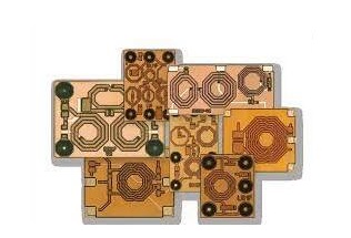


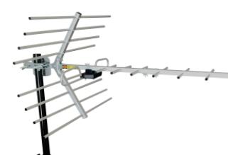

